Abstract
An experiment was conducted to analyze the sound of pickleball paddles and balls upon impact. The goal was to produce a singular parameter that would account for the intensity and quality of the impact sound over its entire duration. Two composite parameters were constructed — the "structure coefficient" and "effective loudness." The purpose was to analyze the relationship between paddle structure and impact sound. Over 100 paddles were tested, as well as several paddle modifications and other impact implements. Up to a 4 times reduction in effective loudness was obtained by experimenting with various objects or paddle modifications. Effective mass, moment of inertia, and thickness were found to be the dominant contributors correlating to the produced sound. Though stiffness is critical, all paddles were so stiff that differences in perceived sound were not correlated to slight stiffness variations. It was found that the effective loudness parameter is very strongly correlated with the sound pressure maximum parameter.
Note: There are lengthy "Paddle Acoustics 101" sections to introduce the experiment. To jump directly to the experiment, click here: GO TO EXPERIMENT.
1. Introduction
The impact of a pickleball ball and a paddle typically produces a short, loud, high-pitched sound. Given that many pickleball courts are located close to residential areas, this can create noise-annoyance situations. Much study, effort, and money have been directed toward solving this problem. Various sound attenuation plans and methods have been developed. These techniques aim to reduce the average loudness level to that of general environmental noise. This goal can be approximated by increasing the distance from courts to residences (on new builds), constructing barriers, employing sound attenuation fences, limiting time of play, requiring play with neighborhood or resort-approved "quiet" paddles and balls, and designing quieter paddles and balls. This study is concerned with this last option — what can be done about the sound itself before it needs mitigation? Can it be reduced or modified at the source without sacrificing performance or the aesthetic enjoyment of the game? Changing the nature of the impact sound first requires understanding that sound. Even when measured as equally loud, each paddle is perceived as sounding more or less annoying than others. Every paddle has a signature sound profile. Understanding the causes and mechanisms of that difference is key to modifying the sound. That is the primary aim of this research.
2. Loudness
A gun shot records a loudness of 140 dB, a rock concert 120 dB, the sound of a pickleball hit is 90 dB, and a car driving by at 60 mph is 70 dB. Even if you don't know what a decibel (dB) is, you know that 140 is greater than 120 is greater than 90 is greater than 70. And, given the numbers, you probably also automatically figure that a gun shot (140 dB) is twice as loud as car noise (70 dB). If only it were that easy.
Loudness is a perception; it is not a unit like meters, mass, or time. It is not an absolute measurement or property of sound. A pickleball impact is a physiological response to vibration in the air that is subjective and different for every person. The processed, perceived sound is not the same as the physical stimulus sound. What a person hears depends on the anatomy, physiology, and health of the auditory system. In addition, sound perception is intertwined with evolutionary adaptations, emotional overtones, and cultural meanings that all get included in the interpretation and "quantification" of all that we hear. Two analytical descriptions of sound processing help to illustrate how and why perceived loudness is subjective and not an exact reproduction of the physical signal — (1) equal loudness contours and (2) non-linear auditory processing. These are a consequence of the physics and physiology of human auditory processing. A discussion of these follows.
2.1. Equal loudness contours (Fletcher-Munson curves)
The physical magnitude of an air pressure variation can be measured precisely; the perceived magnitude cannot, but it can be perceptually scaled and mapped based on the statistical analysis of a multitude of experiments. Experimental subjects are presented with two sounds — the reference sound of specific intensity at 1000 Hz, and a second test sound. The test sound is played at given frequencies, and its intensity is adjusted until its perceived loudness is equal to that of the reference tone. This procedure is then repeated at many frequencies, and the equal loudness intensity for each test frequency is plotted on a loudness vs. frequency graph. The intensity of the 1000 Hz reference tone is then changed, and all frequencies are again compared to the new reference tone. Points of equal loudness to each given reference intensity are then connected by lines, creating the "equal-loudness contour map" (Figure 1).
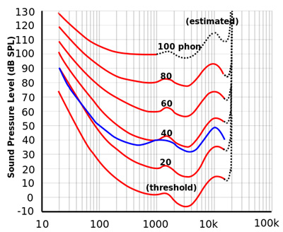
Figure 1 — ISO-226:2003 Equal Loudness Contour Map (Lindosland, Public domain, via Wikimedia Commons). The blue line is an example of the original 1933 Fletcher-Munson results, and the red lines are the ISO-226:2003 revisions based on recent research. The numbers attached to the curves are known as "phons". A phon is the perceived loudness as determined by a group of test subjects of any given sound intensity at 1000 Hz. For example, any sound lying on the 40-phon curve means that it is perceived of equal loudness to a 1000 Hz reference tone presented at 40 dB. That means that the sound has a loudness of 40 phon even though the physical sound pressure on the ear is different. The same reasoning applies to each curve. It is important to note that the perceived loudness values as represented in phons on the curves is not the same as the actual physical loudness as represented on the y-axis. More detailed maps are available showing contours for a much greater range of sounds. All sounds are presented to subjects as pure, continuous sounds (i.e., not impact sounds, such as impact of a ball and paddle) .
The map shows how perceived loudness depends on both frequency and intensity. The loudness contours are a mapping of the perceived sounds to measured physical sounds. For example, on the contour line marked 60, the intensity of a 100 Hz frequency must be at a physical intensity of about 78 in order to be perceived as loud as a 1000 Hz frequency with a physical intensity of 60. Every point on a given line corresponds to an equal perceived loudness to that of 1000 Hz at the line's labeled phon value. Any part of the 60 contour line that is above the horizontal line drawn from 60 (or any other value) on the y-axis indicates that the ear is less sensitive at those frequencies, and anywhere the line is below 60, the ear is more sensitive. Another way of interpreting this is that a 60 dB, 100 Hz sound would be perceived as less loud than a 60 dB, 1000 Hz sound, even though they are of the same physical intensity.
As noted in Figure 1, the direct 1-to-1 mapping of complex impulse sounds, like pickleball impacts, to the figure's pure, continuous, sound-generated curves is perhaps a bit tenuous. In addition, there is a paradoxical observation concerning the contour map. The frequencies that are frequently accused of being the noise culprits occur around 1200 Hz. At that frequency, there is an upward bump that exists on all the contour curves that interrupts the downward slope of the curves. This indicates that the ear is less sensitive at those frequencies within the bounds of the bump and that it takes greater stimulus to be perceived as equally loud as the same stimulus intensity at 1000 Hz. But all that aside, the equal-loudness contours are none the less instructive and relevant to understanding auditory processing. The main point is that people perceive sounds of equal physical intensity to have a different loudness depending on frequency. This is also true of pickleball, but short, impulsive impact sounds present unique challenges in analysis and interpretation.
2.2. Non-linear auditory processing
If the sound stimulus is doubled in intensity, intuition expects that the perception of its loudness will also double. In fact, due to humans' auditory processing, it takes ever greater changes in signal strength to elicit equal perceived changes in loudness (Figure 2). Experiments have shown that, as a "rule of thumb," to approximately double the perceived loudness of any given sound, you have to multiply the stimulus pressure by 10. And to double that result, also multiply it by 10, and to double that, multiply by 10 again, and so on. We have to increase the air pressure 10 x 10 x 10 = 1,000 times to double the perceived loudness three times (i.e., 2 x 2 x 2 = 8 times the initial loudness). The physical sound signal increases exponentially by powers of 10, while the perceived loudness increases logarithmically (explained in Section 6). This "rule of thumb" applies most accurately for sounds at 1000 Hz, and slightly less so otherwise.
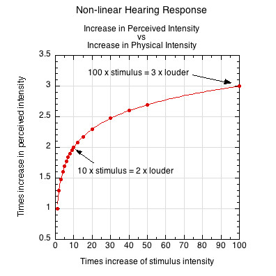
Figure 2 — Non-linear response to sound stimulus increase. It takes greater and greater increases in physical intensity to produce equal differences in perceived loudness increase. For example, 10 times the original stimulus produces a perceived loudness of 2 times as loud. Multiplying the original stimulus by 10x10, or 100, produces a perceived loudness of 3 times as loud as the original. And to produce a sound 4 times as loud as the orignal sound, you have to increase the original stimulus 1000 times.
Non-linearity does not mean that there are gaps in hearing. Hearing itself is continuous in the sense that all frequencies and intensities within the hearing range will produce sound. It is the perception of the change in sound that gets flattened. To see why, we must briefly examine auditory physiology.
3. The Physiology of Sound
Perceived loudness depends on frequency and intensity, but the sensitivity to that dependence decreases as stimulus intensity grows exponentially. This is due to the structure and operation of the ear's "measuring" apparatus.
The ear converts air pressure into electrical signals. In a perfect, synchronized world, the electrical signals produced by the microphone and ear would be exact linear reproductions of each other. Instead, the conversion of sound into electrical signals in the ear proceeds through a series of biological processes that selectively shape, encode, and preprocess sound for further processing in the brain.
This process occurs as follows: The ear pinna (outer ear) collects the vibrating air and funnels it down the ear canal to the eardrum, or tympanic membrane. The pressure waves cause the eardrum to vibrate. Three very small (smallest in the body) bones are attached to the other side of the eardrum and vibrate with it. These bones, the malleus (hammer), incus (anvil), and stapes (stirrup), terminate on the snail-shaped cochlea, or inner ear. Together, these bones are called the ossicles.
The ossicles perform the function of increasing or amplifying the pressure. This occurs because the force is transmitted from a large area of contact with the ear drum to a smaller contact area with the cochlea. A force over a smaller area creates more pressure. This increased pressure is needed because the cochlea is filled with fluid instead of air and requires more pressure to be set into motion.
The liquid's vibration causes pressure waves in the fluid. These waves interact with the basilar membrane, which travels the length of the cochlear channel. The membrane varies in thickness and stiffness, so each section of the membrane will have varying reactivity to the fluid frequency vibrations. The lower section of the membrane is stiffer and thinner, making it sensitive to higher frequency pressure waves. The upper end is thicker and softer and is set in motion with lower pressure waves.
It is physiologically impossible to tune the basilar membrane response to every frequency. Instead, it is sensitive to ranges of frequencies ("critical bands"), which are treated as a single bundled sound. The size of these critical bands also varies — narrower for low frequencies and wider for higher frequencies. Hair cells are located throughout the cochlea and are attached to the basilar membrane. These hair cells wave in the fluid when the membrane is set in motion. Specific hair cells are activated according to their location on the basilar membrane. As a result, hair cell and membrane activation occurs specific to the frequency of the fluid pressure waves. The movement of the hair cells generates ions that travel down the hair bundle to the bottom of the hair cell, causing the release of neurotransmitters. The neurotransmitters bind with the cells of the auditory nerve and create an electrical signal that travels to the brain. The nature of that signal depends on which hair bundles were stimulated.
Finally, the brain interprets the signals. This entire process filters, masks, augments, and attenuates the intensities of specific frequencies. As such, it is a non-linear process — 10 times the stimulus intensity does not lead to 10 times the perception. Nonetheless, it is a process that evolution has selectively settled upon to optimally adapt to our acoustic environment and the survival context in which it is embedded.
4. Sound Measurement
Understanding sound requires some knowledge of how it is measured and analyzed. Sound is caused by pressure variations in the air. If you clap your hands or hit a ball with a pickleball paddle, air is quickly compressed between the two objects and pushed out in all directions. Compression pushes air molecules closer together, causing higher pressure. The faster the impact, the greater the compression and pressure. These molecules push into adjacent molecules, compressing them, whereupon they rebound in decompression (or rarefaction). The pressure wave continues outward with its chain reaction of compression and rarefaction, with molecules oscillating about their equilibrium positions. The wave travels, but the individual molecules do not, with the exception of oscillations about their equilibrium positions.
The pressure wave reaches a measuring device, where its strength (amplitude) is measured. Microphones measure the movement of a diaphragm that is instrumented to convert physical motion into electrical signals with a voltage proportional to the diaphragm's displacement. This signal is passed on to digital processing devices that analyze many representations of the sound waves. Three such representations are generated by the sound meter (peak loudness view), the oscilloscope (time domain view), and fast-fourier transforms (frequency domain view). Each view offers a different perspective on the sound.
4.1. Sound Meter
Sound meters measure loudness, but that measurement is complicated by the fact that human hearing is not additive. It does not just add the pressure at each frequency to get the total pressure and loudness. The ear is not equally sensitive to all frequencies. It is maximally sensitive between 2,000 and 5,000 Hz, and below and above that, it has a reduced resolution to its “measurements” of pressure and loudness. So what we hear depends on this biological filtering, not the sound's physical reality. Sound meters apply frequency weighting filters to the raw sound pressures to mimic the ear's sensitivity to certain frequency ranges. They achieve this by attenuating the sound signal from lower and higher frequencies and amplifying those to which the ear is most sensitive. In that way, the sound meter loudness value more nearly represents our perception of sound level, not the actual physical level.
Sound meters have three primary frequency weighting settings. The "A" frequency setting attenuates lower frequencies (< 500 Hz) to the greatest extent and a smaller amount at higher (> 6000 Hz) frequencies. The "C" setting filters the same range of frequencies as does A, but less so. The "Z" setting does not filter any frequencies. The experiments below were conducted using the C setting.
So, loudness perception depends on the sound’s dominant frequencies and the pressure level of each of those frequencies. It also depends on the sound's duration. Sound meters also have settings that determine the time frame within which sound calculations will be averaged. These are "slow" (> 1 s), "fast" (125 ms), "impulse" (35 ms), or "equivalent continuous" sound (Leq), which averages sound over a user-defined time. All settings will capture the instantaneous peak, but other measurements will average over the different durations. The experiments below were performed with the impulse setting.
The actual duration of a pickleball paddle/ball impact is about 2 ms, much shorter than any of these settings. However, the ear does not just hear the actual impact but also packages up to 30 ms of post-impact air vibration sound into that singular impact sound. Both paddle and ball continue to vibrate and those vibrations continue to produce sound. The ear integrates a significant portion of that continuum into one discrete perception of impact.
Frequency weighting is complicated by the fact that an impact is so short —too short, in fact, for the dominant frequencies of the paddle and ball to be determined during contact. Each object's deformation wave needs sufficient time to travel the full dimensions multiple times to establish their vibrational wave forms. That being the case, as well as the fact that most pickleball impacts are loud and involve substantial amounts of lower frequencies, it is best to set the sound meter to the C setting. That accounts for both the lower resolution of frequency modalities at the beginning of the impact and for the determination of their post-impact resolution and contribution.
Though quick, easy, and ubiquitous, sound meter measurements of loudness, by themselves, do not give us much insight into the nature and make-up of a sound. This is important because sounds measured equally loud are not necessarily perceived as having the same loudness, quality, or timbre. Two tools used to more comprehensively analyze sound are the oscilloscope and the Fast-Fourier Transform (FFT). The oscilloscope records the sound pressure at every instant. The y-axis is presented in either volts or Pascals (Pa), and the x-axis in time (therefore, called the time domain view). The FFT (frequency domain view) shows frequency on the x-axis and pressure on the y-axis. Together, these two views display sound pressure over both time and frequency, allowing us to pinpoint the concentration of sound energy. That leads to determinations of the properties of the ball and paddle, which, in turn, tell us where and how materials and design can be altered to influence the sound.
4.2. Oscilloscope
When the sound wave signal is passed to an oscilloscope, it displays a graphical representation of the pressure wave on screen, showing its peaks (compressions) and valleys (rarefactions) measured in Pascals (N /m2) over time. A Pascal is a measure of force per area. One such wave is displayed in Figure 3. This is a graph of a ball traveling 3.8 m/s and hitting the center of the paddle (as are all graphs with the label "VARIN," which is the Tennis-Warehouse product code for the Selkirk Vanguard Power Air Invikta MW paddle).
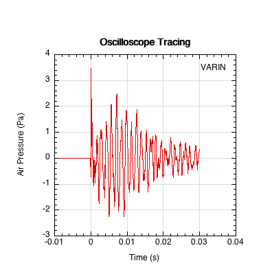
Figure 3 — Oscilloscope tracing of a Selkirk Vanguard Power Air Invikta MW. Only 30 ms of sound was recorded. Often times you will see a longer duration displaying the signal decomposition into background noise, which is characterized by the roughly constant amplitude and broad, non-periodic tracing after the impact. Every oscilloscope capture will include the background and reflective noise in the measurement (unless the measurement is performed in an anechoic chamber).
There is a very steep, transient peak at the beginning of the impact. The initial hit causes an immediate deceleration of the ball, creating a high-force pressure wave. This is represented on the y-axis. The faster the collision and the greater the paddle mass and stiffness, the greater will be the ball deceleration and resulting peak pressure and sound. After the first 3 or 4 ms, the peaks seem to occur at roughly equal time intervals. This interval is the "period" of the pressure wave — the time required for the air pressure to make one oscillation from peak compression to rarefaction and back to peak compression. In the simplest case, the number of these peaks per second is the fundamental frequency of the pressure wave. If the period is 0.0005 seconds (half a millisecond), then the frequency would be 1 second divided by 0.0005 seconds, which equals 2000 cycles per second (CPS, or more commonly, Hz). The actual impact time is only about 2 ms — about 1-2 periods of the oscilloscope trace, or about the first positive inward tick on the x-axis. This is where the peak pressure occurs. However, the next several milliseconds are also incorporated into what we hear. After the initial impact, we hear the sound of pressure waves created by the post-impact vibrations of both the paddle and ball. It is in this post-impact region that the various frequencies of the sound establish themselves to bring us timbre and pitch, two very important ingredients to our perception of loudness. But these frequencies are often difficult to decipher from an oscilloscope trace.
4.3. Frequency Spectrum FFT
A mathematical procedure known as a Fast Fourier Transform (FFT) converts the oscilloscope's time domain view into a frequency spectrum domain. The FFT graph plots pressure on the y-axis and frequency on the x-axis. This shows how much pressure is associated with each frequency (Figure 4).
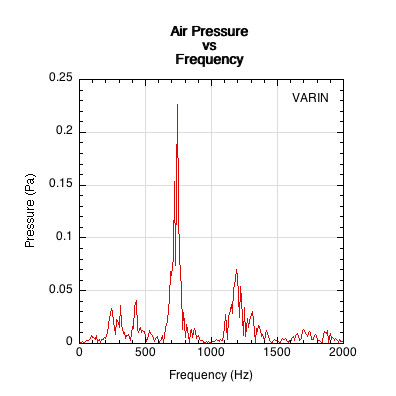
Figure 4 — Air pressure vs. frequency. The pressure responsible for all those squiggly lines in Figure 3 is concentrated in just a few frequencies. The maximum frequency on the x-axis is 2,000 Hz because no higher frequency was elicited from any ball-paddle impacts.
5. Sound Pressure Ratios
5.1 Reference Pressure Ratio
The pressures given in Figures 3 and 4 are for the physical impact event, but humans are only capable of hearing a limited range of measurable pressures and energies (due to many factors discussed in Section 3). To make the pressure measurements relevant to human hearing, all sound pressures are compared to the threshold of hearing, which is traditionally accepted to be 20 µPa (also written as 0.00002 Pa, or 20 x 10-6 Pa) and referred to as \(p_{ref}\) or \(p_0\). Every sound pressure \((p)\) is divided by this “reference” pressure to create the sound pressure ratio \(\frac{p}{p_{ref}}\). This ratio ranges from 0 to 10 million or more times the threshold of hearing. Figures 5-7 show different views of the pressure ratio. Figure 5 shows a graph of the relationship between the absolute physical pressure and the relativized pressure ratio over a very large range of sounds. Figure 6 shows a cut-out of the region containing an example of the ball traveling 3.8 m/s and hitting a stationary pickleball paddle. Figure 6 would be located in the very bottom left corner of Figure 5. Figure 7 shows the pressure ratio plotted against frequency for the same ball/paddle impact.
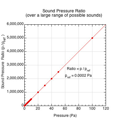
Figure 5 — Pressure Ratio. All sound pressures are compared relative to the threshold of sound (20 x 10-5 Pa). Pressure ratios can range from 0 to millions of times the threshold pressure.
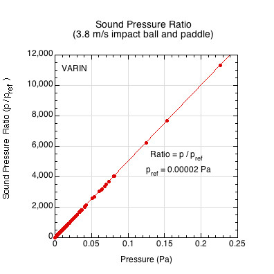
Figure 6 — Pressure Ratio for the paddle impact example. This graph is a zoomed portion of Figure 5 where it would be located in the very bottom-left corner.
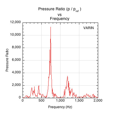
Figure 7 — Pressure Ratio vs frequency for the paddle impact example. This graph looks very similar to Figure 4 which was a pressure vs frequency plot. The difference is that Figure 4 was an absolute plot — i.e., the plotted values on the y-axis are all of the raw, physical event. The graph here is a relative plot — all the y-axis values are relative to the threshold of hearing.
A ratio is one quantity divided by another and represents a comparison such that one value is "x times" larger or smaller than another. The pressure ratio quantifies sound pressure in terms of how many times it is greater than the threshold pressure. If the quantities have the same units, as is the case here (Pa), the units cancel and the ratio is unitless. The pressure ratio converts absolute measurements of the physical event into relative comparisons to a reference event.
5.2 Pressure Ratio Squared and Energy
But the pressure ratio by itself has a limited value. Though pressure is easy to measure and intuitively and perceptually familiar to most people, it is just a means to get to what we are really interested in — the energy, power, and intensity of the pressure wave. Sound energy manifests as moving and vibrating particles of air (kinetic energy), as well as the potential energy stored in its compression and rarefaction. It is the moving particles that create the pressure. The moving particles are the fundamental carriers of sound. Regions of high pressure indicate more intense particle vibration and energy transfer between particles. Energy is measured in joules (J). Power is the rate at which energy is transferred and is measured in Watts (W), which is energy per unit of time. Intensity is the power per square meter and is measured as \(\frac{W}{m^2}\). Intensity, then, is the amount of energy transferred per unit of time per square unit of area. This gives us the most comprehensive picture for analyzing the properties of the physical sound and its auditory perception. That being said, it should be remembered that energy is the underlying explanatory concept upon which pressure, power, and intensity depend. Because all four concepts are related, it turns out that we can move between them by considering the square of the pressure measurement. Power and intensity are both proportional to pressure squared (e.g., \(I \propto p^2\) and \(P \propto p^2\), where I is intensity and P is power). For that reason, we perform most analytical calculations with pressure squared and pressure ratio squared. Up to this point, our analysis has been descriptive of the physical event in terms of pressure. But pressure is itself simply the result of the transfer of energy over time and space. It is the proportionality between pressure squared and power that allows us to examine this flow of energy and move from description to analysis. Figure 8 shows pressure ratio squared vs. frequency, and Figure 9 shows pressure ratio squared vs. pressure.
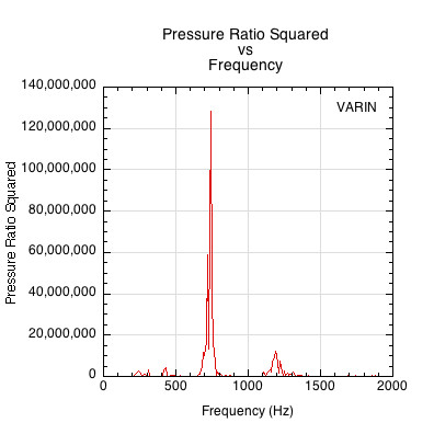
Figure 8 — Pressure ratio squared vs frequency.
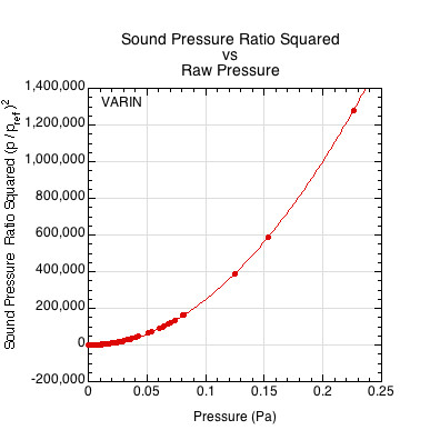
Figure 9 — Pressure ratio squared vs pressure.
6. Introducing Logarithms, Bels, and Decibels
It is apparent from looking at the y-axis values in Figures 8 and 9 that squaring the pressure ratio results in very large magnitudes — up to 100 trillion. We obviously don’t perceive sound in gradations of trillions, nor do we want to calculate with such large numbers, so we compress the measurement scale into powers of 10 in order to make it more usable and meaningful. We do this by asking, "What power (exponent) of 10 equals the pressure ratio squared?" The mathematical representation of this question is
\begin{equation} y = log_{10}\left(\frac{p}{p_{ref}}\right)^2 \end{equation}Alternatively, we can use the power ratio instead of the pressure squared ratio:
\begin{equation} y = log_{10}\left(\frac{P}{P_{ref}}\right) \end{equation}Where \(y\) is the power, or exponent, p pressure, and P power. The subscript "10" is the base we are raising to the power of y. The power law of logarithms brings the exponent out in front of the logarithm. Thus, the logarithm of the pressure ratio squared is 2 times the logarithm of the pressure ratio as shown in Equation 3.
\begin{equation} y = 2log_{10}\left(\frac{p}{p_{ref}}\right) \end{equation}Equations 2 and 3 are equivalent methods of achieving the same result. The graph in Figure 10 shows how these very large pressure ratio values are compressed into very small logarithmic units (actually, each unit is still a ratio in the sense that it represents "10 times" the value of the previous logarithmic unit). The pressure ratios squared are on the x-axis, and the compressed logarithmic values of those are on the y-axis (sound pressure level or SPL axis).
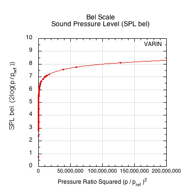
Figure 10 — bel scale: Logarithm of pressure ratio squared for ball hitting paddle. Y-axis values are the exponents to which 10 must be raised in order to equal the corresponding value on the x-axis. On a logarithmic scale, the pressure is referred to as "sound pressure level" (SPL) to indicate that it is not a raw measurement but a relativised, scaled measurement. The graph curve fit here is characteristic for logarithmic pressure plots — larger and larger increases in x-axis values are necessary to achieve equal percentage change in the y-axis values.
The y-axis is now logarithmic. The y-axis labels are the logarithms of the x-axis values (pressure ratio squared), or, in other words, the exponents to which 10 is raised to equal the corresponding x values (pressure ratio squared). Now the y-axis values are relative, logarithmic, unit-less ratios. This ratio is referred to as the sound pressure level (SPL). At this stage, each tick on the scale is known as a "bel" (after Alexander Graham Bell). This, then, is known as a bel scale. The shorthand nomenclature is SPL bel, meaning the sound pressure level scaled in bels. We have compressed our huge pressure ratio squared numbers on the x-axis into workable numbers on the y-axis, where every one unit increase is equal to a 10-fold increase in magnitude.
But describing sound in only 10-time jumps lacks detail, so the bel scale is multiplied by 10 to create a new scale — the decibel scale. Mathematically, Equation 2 is multiplied by 10, resulting in Equation 4. This equation is the standard formula for converting pressure to a sound pressure level in decibels. Figure 11 shows the standard graphical representation plotting SPL dB vs. pressure (lower case p).
\begin{equation} y = 20log_{10}\left(\frac{p}{p_{ref}}\right) \end{equation}Or, using the power (upper case P) ratio instead of the pressure squared ratio:
\begin{equation} y = 10log_{10}\left(\frac{P}{P_{ref}}\right) \end{equation}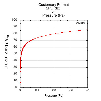
Figure 11 — Customary presentation of SPL dB vs pressure (Pa) The y-axis is calculated using the square of pressure on the x-axis, as explained above.
A logarithmic scale is simply a different way to write numeric values. It does so by representing each measured value, x, as the power to which 10 must be raised to equal x, or, in other words, what value of y makes \(10^y\) equal to the value of x? That number, y, can then be used as a scaled representation of the original number, recognizing that the original value is not the exponent but 10 raised to the exponent. The original value is still there, but it is just in an "encoded" form. When placed on an axis, each "unit" increase in y, the exponent, represents a 10 time increase of the previous unit — in other words, going from 2 to 3 on a graph axis would mean going from \(10^2\) to \(10^3\), which is 10 times \(10^2\) = \(10^3\), or 10 x 100 = 1,000. Equal increments along a logarithmic scale are equivalent to 10-time increments of the original value.
It is frequently said that human hearing is logarithmic. This is correct, but it is not, as is sometimes mistakenly thought, because the physical event is measured on a logarithmic scale. It is because of the way we physiologically and conceptually process sound, as discussed in Section 3.
7. Energy, Power, and Intensity
The decibel scale is usually associated with loudness. When speaking about the pickleball noise problem, most people refer to the SPL dB level. And then all paddles are compared relative to this number. But this number does not tell us much about the perceptual contents of the sound. Examining sound in terms of its energy, power, and intensity at each frequency is crucial to understanding our perception of the sound. Energy, power, and intensity are all intertwined with each other. Energy (E) is the capacity to produce a change in a physical system due primarily, in our case, to a system's motion or position. Energy is measured in joules (J), so \(E = \frac{kg \cdot m^2}{s^2}\). Power (P) is a measure of how fast this energy is being used to produce change. It is measured in Watts (W), which is energy (joules) per second (\(P = \frac{kg \cdot m^2}{s^3}\)). Intensity is power per unit area (A, or \(m^2\)), so \(I = \frac{P}{A}\), or energy per second per area. Because power is directly proportional to the square of pressure, which is our primary sound measurement, we will utilize it to more deeply explore the nature of impact sound.
The equation for intensity is \begin{equation} I = \frac{p^2}{\rho \cdot c} \end{equation} where \(p\) is the pressure, \(\rho\) is density of the air and \(c\) is the speed of sound in air. This equation reflects the strength of pressure changes and how efficiently the air can transmit those changes due to its density and the speed of sound in air.
Replacing each variable with the fundamental SI units from which it is derived, the equation becomes \begin{equation} I=\frac{kg^2 \cdot m^2 \cdot s}{kg \cdot m^2 \cdot s^4} = \frac{P}{m^2} \end{equation} A unit analysis of this equation shows that all the requisite units for energy, power, and intensity are present. However, since intensity is power/area, and area in our case is one meter squared which is equal to one, then intensity effectively reduces to power. \(I=P\), when \(A=1\). Our calculations are based on this simplification.
7.1. Power Spectral Density
Next we want to plot power vs frequency, but first we want to normalize power per unit of frequency. The FFT software calculates power data averaged over every 10 Hz. Dividing the power value by 10 will give the power per unit of frequency over each 10 Hz "data bin". Figure 12 plots frequency-normalized power vs frequency.
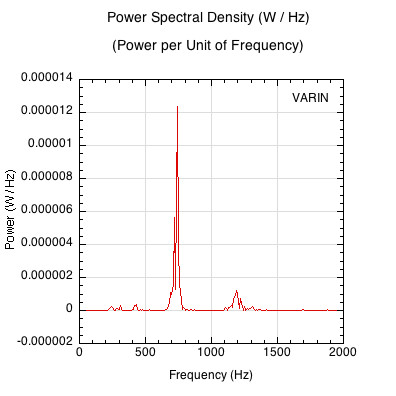
Figure 12 — Power Spectral Density Graph Normalized For Frequency. The power associated with each unit of frequency from 0 to 2000 Hz.
The y-axis units are the absolute power values. By themselves they have little contextual meaning. We can further normalize the individual power values by expressing them as a percentage of the total power (i.e., here, "percentage" means "relative to the total") over this range of frequencies. We refer to this as "relative power spectral density" because the value of each data point is the percentage of the total power consolidated into each Hz. This view renders precise frequency locations of the total power as well as the relative magnitude at each location. Figure 13 shows this.
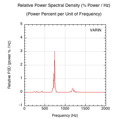
Figure 13 — Power Spectral Density Graph Normalized for Frequency and Power. The relative percent of total impact power associated with each unit of frequency.
Figure 13 shows the percent of total power at each unit of frequency. This is a very striking representation of where and how much of the total energy of the impact is concentrated. We can go one step further and show the cumulative total energy of the impact as it sums over all frequencies. Plotting the integral (summation) of the relative PSD over the frequency range from 0 to 2000 results in Figure 14. The y1-axis represents the
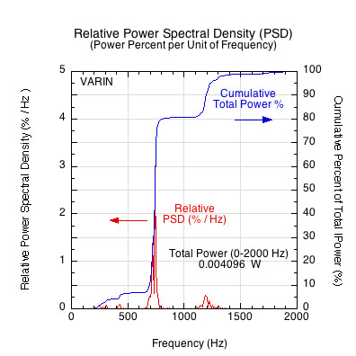
Figure 14 — Power Spectral Density Graph Normalized for Frequency and Power. The relative power per unit of frequency and the cumulative percent of total power accumulated from 0 to the specified frequency. As can be seen, 80% of the total power is contained in frequencies less than about 750 Hz.
This analysis become even more striking when impacts on different paddles are compared. Figure 15 shows a comparison of relative power spectral density graphs of 4 paddles.
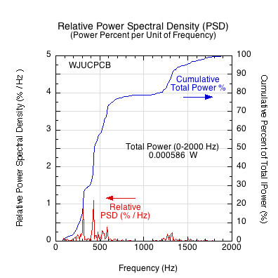
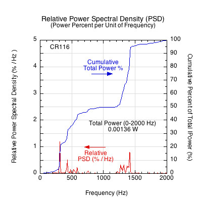
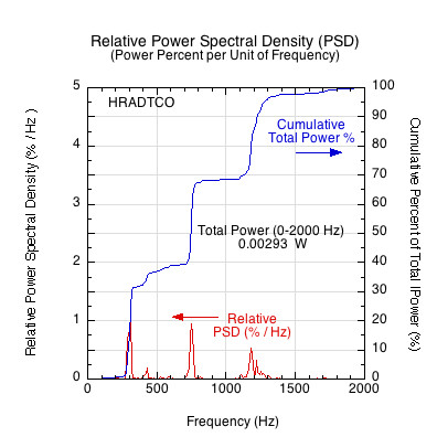
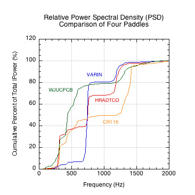
Figure 15 — Comparative relative power spectral densities. Each curve shows the percent of total power contained over all frequencies. Many paddles concentrate power at similar frequencies but do so with varying magnitudes.
Figure 15 shows what percent of the total power is concentrated at each frequency. Figure 16 shows the cumulative total raw power contributed at each frequency. Figures 15 and 16 together show the importance of both the power magnitude and location.
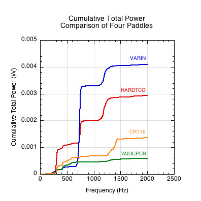
Figure 16 — Paddle comparison of total sound power vs frequency. The location and magnitued of power concentration is evident for each paddle. Interestingly, all paddles have a similar frequency profile but vary in the magnitude of power at each frequency.
7.2. Power Spectral Centroid and Spread
Power spectral density is a great tool for visualizing the location and magnitude of the acoustic power on the frequency spectrum. However, we can still zoom in further to get more detailed and singular descriptions of the impact sound. What we really want is a single number that captures how the physical properties of the paddle contribute to the impact sound. The peak sound meter number is often used, but this is much too transient, and it does not correlate to any physical property of a paddle.
The FFT shows the amount of each frequency present in a sound, and the amplitude of each frequency is a proportional representation of the distribution of energy. It is useful to calculate the power spectral density (PSD) centroid, or, the "center of mass" of the power spectrum (it is also the center of energy of the sound, since power is energy per second). This is represented as the PSD centroid and is calculated as
\begin{equation} C = \frac{\sum_i{f_i(S_{fi})}}{\sum_i{S_{fi}}} \end{equation}where C is the PSD centroid, fi is a particular frequency in the spectrum, and Sfi is power per Hz amplitude of that frequency. This calculation is in Hz, and it is the center of power of the sound. The spectral centroid is the average of all frequencies in the sound, weighted by their amplitudes. The centroid is a single number that indicates both the magnitude and distribution of the sound's energy.
Spectral spread is a similar number. Effectively, it is the standard deviation of the PSD around the PSD centroid, indicating how spread out the energy is about the centroid. The formula for the PSD spread, \(\sigma\), is given as
\begin{equation} \sigma = \sqrt{\frac{\sum_i{(f_i-C)^2(S_{fi})}}{\sum_i{S_{fi}}}} \end{equation}where (\(f_i-C)^2\) is the squared PSD difference of each frequency component from the centroid and \(S_{fi}\) is the PSD amplitude at each frequency. A wider spread indicates a richer, more complex array of frequencies, and a narrow spread would indicate a purer, simpler sound.
Both the PSD centroid and spread are valuable singular values that aid in comparing the sound of different paddle impacts, but we will see later in Section 8 how to combine them with the physical properties of the paddle to uniquely describe its impact sound.
8. The Experiment
One hundred and ten paddles were tested. The aim of the experiment was to measure and characterize the sound of a colliding paddle and ball, compare the sounds of all paddles, and determine which paddle properties were most important to influencing variations between paddles.
A Selkirk Competition outdoor ball was dropped as a pendulum from 72 cm above the center of the paddle face (Figure 17). The impact speed was about 3.8 m/s. The paddle was suspended by a string from the end of the handle. This allowed the impact to be determined by the true acceleration, mass, stiffness, and vibrational modalities of the paddle, independent of any support structures. A MicW i436 microphone was placed one meter from the impact location, about 45 degrees in front of the paddle. The signals were processed by the Faberacoustical SignalScope X software package. Data from SignalScope X was then exported to KaleidaGraph graphing software for further analysis.
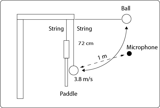
Figure 17 — Experiment setup to to measure sound of paddle and ball impacts. The ball is dropped from 72 cm above impact point on the middle of the paddle face. Ball velocity at impact is 3.8 m/s. The microphone is located 1 meter from the impact point.
To determine which physical properties of the paddles correlated with the properties of the impact sound, measurements and calculations of both were performed. The relevant paddle properties were thickness, stiffness, weight, balance, swingweight at 10 cm (moment of inertia, I10), apparent coefficient of restitution (ACOR), and effective mass, Me, where \(M_e = \frac{MI_{cm}}{(I_{cm}+Mb^2)}\), b is the balance point, and Icm is the moment of inertia about an axis at the center of mass. Sound properties measured were peak sound pressure level (SPL peak), sound pressure level maximum (SPL max), fundamental frequency, frequency spectrum, energy, power, intensity, power spectral density (PSD), PSD centroid, and PSD spread. All measurements and calculations were made between 0 and 2000 Hz and over a duration of 30 ms. There were no significant contributions to sound power above 2000 Hz, and the impact sound dampens to general noise beyond 30 ms or less.
8.1. Comparing Impact Loudness
The first and most striking finding was that all paddles are loud, and on average, they all have about the same level of loudness. Peak sound levels were between 99 and 106 decibels. However, as discussed, measured loudness and perceived loudness are not identical. The difference in perceived loudness between 99 and 106 decibels can be shown in two ways. The simplest, least rigorous method is to use Equation 10, which is derived from Equation 5 using the psycho-acoustical observation that a 10 dB increase in sound pressure level (SPL) is roughly equal to a doubling in perceived loudness.
\begin{equation} L = 2^\frac{dB}{10} \end{equation}Where L = perceived loudness, dB is the difference between the upper value (106) and the lower value (99). So \(L=2^\frac{7}{10} = 1.62\). The 106 Hz peak SPL is 1.62 times the 99 Hz. If the dB difference was 10 dB, then the equation would be \(L=2^\frac{10}{10} = 2\), or double, as expected.
The other more accurate method of determining the perceived loudness difference of this range between 99 and 106 Hz is to use Stevens' Power Law:
\begin{equation} \sigma = k(I-I_0)^n \end{equation}Where σ is the loudness multiplier, I is intensity, I0 is the reference intensity being compared to, n is the exponent, and k a scaling factor. The n and k are empirically derived and adjusted as necessary to meet experimental conditions and results. Using the common values of n = 0.6 and k = 0.5 for illustrative purposes, we get σ = 1.61. In other words, and similar to the results of Equation 10, 106 Hz will be perceived as 1.61 times as loud as the 99 Hz sound. If, instead, there was a 10 dB difference between I and I0, σ = 1.99, or, as expected, a perceived loudness difference of two times louder than the lesser reference intensity.
A 1.61-fold difference in perceived loudness is significant. However, if you live next to a pickleball court, both 99 Hz and 106 Hz "measure" as "too loud." Nonetheless, if paddles are to be manufactured to be quieter, the relevant properties that need modification must be determined. Given the construction of most current paddles, there is little significant difference in properties. There is enough, however, to determine some general correlations between certain paddle properties and sound properties. This is only true if we consider the total power of the sound duration, not the peak sound level. There was no correlation at all between any paddle property and the peak sound pressure level. Normally, it would be expected that there would be a correlation between paddle surface stiffness and peak sound, but all the paddles (by the rules) are similarly stiff. The stiffness was measured by dropping a 1.18 kg mass from 20 cm onto a clamped paddle and measuring transverse deformation and bending. The ball was not included. Perhaps measuring combined ball/paddle stiffness would produce a meaningful relationship between stiffness and peak loudness.
8.2. Paddle Structure Contributions To Sound
The three physical paddle properties that were correlated to the total sound power were thickness, effective mass at impact location, and moment of inertia (swingweight). The graphs of these relations are shown in Figures 18-20.
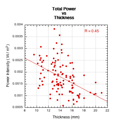
Figure 18 — Total sound power vs thickness.
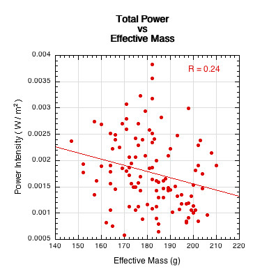
Figure 19 — Total sound power vs effective mass at impact location.
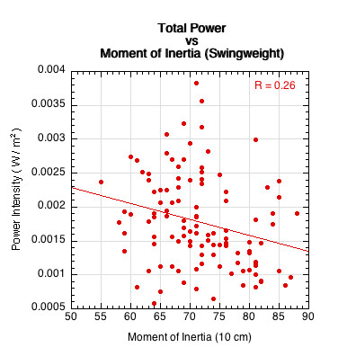
Figure 20 — Total sound power vs swingweight (moment of inertia at 10 cm from butt).
8.3. Paddle Structure and Effective Loudness
The relationships in Figures 18-20 are not very strong, but they have a multiplicative effect when combined into one composite parameter, K, that we will call the "Structure Coefficient".
\begin{equation} \text{Structure Coefficient} = K = \frac{tM_eI_{10}}{10,000} \end{equation}where K is the structure coefficient, t is paddle thickness, Me is effective mass at impact location, I10 is the moment of inertia (swingweight) about the 10 cm axis, and the denominator simply scales the result.
Similarly, we can create a composite sound parameter that is more nuanced and complex than any single parameter, such as power. We will call this composite sound parameter "Effective Loudness" and designate it as Leff. It combines power, PSD centroid, and PSD spread into a more comprehensive acoustic descriptor than do SPL peak or power when considered in isolation. The calculation produces a singular decibel value and is given as
\begin{equation} \text{Effective Loudness} = L_{eff} = 10log\left(\frac{PC}{\sigma P_{ref}}\right) \end{equation}where Leff is the composite effective loudness sound parameter, P is total power, C is the PSD centroid, σ is the PSD spread, and Pref is the power reference value of 1 x 10-12.
Plotting effective loudness, Leff, vs the structure coefficient, K, we find a much better correlation between structure and sound, as shown in Figure 21.
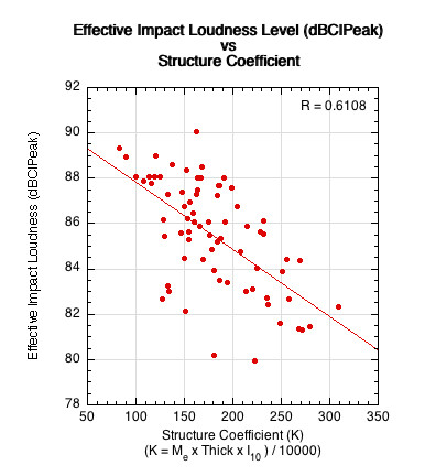
Figure 21 — Effective Loudness The effective loudness is a quantification of the fullness of the sound including its power, frequency, and distribution. It incorporates both the loudness and quality of sound, including "non-quantifiables" such as timbre, "brightness", and "fullness". The structure coefficient includes parameters that influence the force on the paddle and the paddle's absorption, distribution, and transfer of energy.
Tying sound to physical paddle properties allows designers to alter the sound by altering the properties. However, Figure 21 shows that the structure coefficient as composed here is not the full story. It does not account for impact sound. Likewise, the effective sound parameter is not fully inclusive of the total quantity and quality of the sound. But the conclusion of Figure 21 is clear, higher structure coefficient results in lower perceived sound.
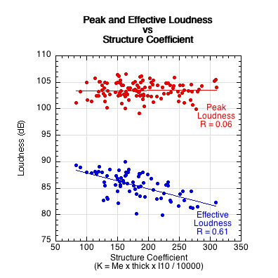
Figure 22 — Peak and Effective Loudness Paddles sound different from each other based on structure parameters such as effective mass, moment of inertia, and thickness.
Figure 22 shows up to a 15 dB difference between a paddle's peak and effective loudness. Using Equation 11, the effective loudness is up to 2.5 times less loud than the peak. The peak loudness is still what it is, but the frequency and quality of the sound surrounding the peak influences a person's perception of the sound. Impact sounds of equal SPL dB can be perceived as louder or softer and more or less annoying than the other depending on the structure of the paddle producing the sound.
8.4. Effect of Mass on Loudness
As the structure coefficient indicates, effective loudness should decrease with increasing mass. To test that directly, various masses were added to the backside of the hitting area, and the sound intensity measured for each added mass. This is displayed in Figure 23.
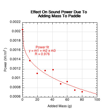
Figure 23 — Effect of adding mass to paddle. Adding mass to the paddle decreases the the total sound power of the impact.
Increasing the effective mass at the impact point influences energy transmission throughout the paddle. Added mass is more difficult to move and vibrate, thus limiting the higher vibrational frequencies and their amplitudes. More mass might absorb more energy and increase the impact duration, stimulating lower vibrational frequencies.
8.5. Effect of Surface on Loudness
Similarly, to test loudness variation based on impact surface material, 3 surfaces were glued to the surface of a paddle — a thin piece of cloth, a piece of tennis ball felt, and a thin (1/4") foam. There was up to a 10 dB difference between the foam and the clean paddle impacts. That is equal to a sound reduction of 1/2. The results are shown in Figure 24.
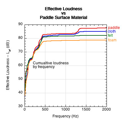
Figure 24 — Effect of the hitting surface on sound. The paddle with foam on the surface was half as loud as the normal paddle (Equations 10 and 11).
Up to about 400 Hz, all surface conditions exhibited very similar effective loudness profiles. Above 400 Hz, the higher frequencies were progressively attenuated with increase in surface material thickness and density. These properties absorbed more sound energy.
8.6. Effect of Hitting Implement on Loudness
Impacts of a pickleball ball were also performed on various objects to see how total structure will influence loudness. Hitting objects were a paddle for reference (234g), Padel racket (346g), wood ping pong paddle with rubber surface (168g), a solid rubber mallet (540g) with wood handle, and a solid 2x4 block of wood (146g). The 2x4 block of wood and the rubber mallet were both about 4 times less loud than the pickleball paddle. Results are shown in Figure 25.
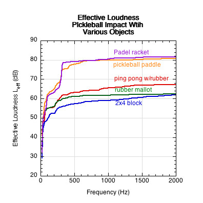
Figure 25 — Effect of hitting object on sound. The 2x4 block was 1/3 (Eq. 11) to 1/4 (Eq. 10) as loud as the paddle.
Wood and rubber appear to very good materials for sound damping.
8.7. Effect of Drilling Holes on Loudness
Varying numbers of 1/4" diameter holes (0, 15, 25, 35) were also drilled in a paddle to see if the sound energy transmission and transfer would be affected. As shown in Figure 26, loudness decreased slightly with increasing hole count.
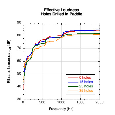
Figure 26 — Effect on sound of drilling various numbers of holes in the paddle. The paddle without holes was about 1.23 times as loud as the paddle with 35 holes.
8.8. Effect of Test Method on Loudness
Different test setups can also influence results. The most common setup is to clamp the paddle at the handle. However, that can alter the paddle properties. Instead, these tests used free paddles (no clamps, hanging from a string) to insure against possible external variable influence on results. Figure 27 shows the clamped paddle has a higher effective loudness.
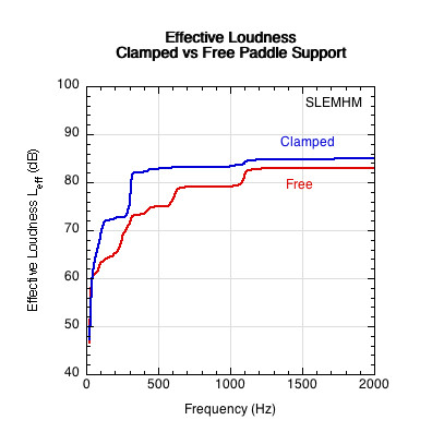
Figure 27 — Effect on sound of clamping paddle or letting it swing free upon impact. The clamped paddle was only about 1.2 times as loud as the free paddle. The free paddle stimulated a broader, more gradual frequency response, whereas the clamped paddle exhibited a steeper, more concentrated response.
Clamping the paddle just above the handle alters the bending modes. It is transformed from a "drum" mode to a "diving board" mode. The handle end is constrained, limiting vibration and also effectively shortening the length. This results in higher stiffness, which in turn causes higher frequency participation.
In general, Figure 28 shows that as the structure coefficient increases, the centroid moves toward lower frequencies, and as the centroid decreases, so does the effective loudness.
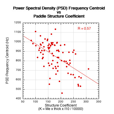
Figure 28 — Power Spectral Density Frequency Centroid. As the structure coefficient increases, the centroid frequency decreases. The centroid is part of the effective loudness equation, so as the centroid decreases, so too does the effective loudness level.
8.4 Relationship Between Effective Loudness and SPL Max
There is a very close relationship between effective loudness and sound pressure level maximum (SPL Max)SPL. SPL Max is calculated using sound meter data, whereas effective loudness is calculated with FFT spectrum data. To calculate SPL rms, the peak average must first be calculated and is given as \begin{equation} p_{peak} = \sqrt{\frac{1}{T}\int_{0}^{T} p^2 \,dt} \end{equation} where T is the duration of the time window (30 ms), p is pressure, and t is the time interval between measurements (about 0.00002 s).
Because the amplitude measurements in this experiment were conducted at peak level type and not RMS, we must convert ppeak to SPLrms, by dividing ppeak by \(\sqrt{2}\) and substitute into Equation 4: \(SPL_{rms} = 20\log(\frac{p_{peak}}{p_{ref}\sqrt{2}})\text{.}\)
SPL Max is a time-weighted pressure measurement whereas effective loudness is a frequency weighted power measure. But because both are proportional to pressure squared, the two results are well correlated, as shown in Figure 29. However, the advantage of effective loudness is that it correlates much better with the structural properties of the paddle (Pearson correlation coefficient: r=0.61 vs. r=0.43; coefficient of determination: 0.37 vs. 0.18, meaning 37% vs 18% of the variation is explained by the model; p-value: p < 0.0001 for both, meaning there is less than one ten thousandth percent chance the relationship is random).
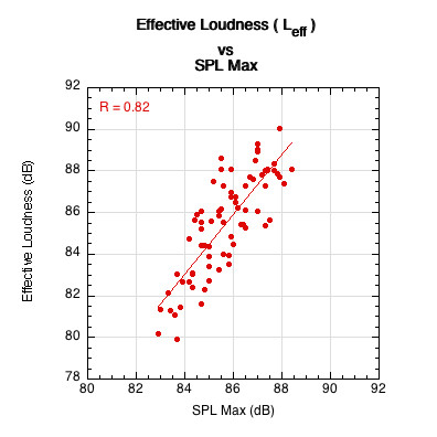
Figure 29 — Effective Loudness vs SPL Max (sound pressure level maximum).
9. Conclusion
The relationship between the composite structure coefficient and the effective loudness parameter demonstrates the viability and predictability of each. Effective loudness successfully quantifies the magnitude, location, quality, color, and brightness of sound into a singular number. Together, the two composite parameters are helpful in understanding and analyzing impact sound.
However, as currently constructed, the relationship between these two parameters still contains unexplained variance. Including additional properties in the structure coefficient might be useful. An appropriate paddle stiffness test is necessary. The stiffness test used in this experiment did not yield meaningful correlations, and investigations into other methodologies are required. The alternate materials, modifications to structure, and objects used in the experiment all reduced effective loudness. As a result of the modifications, variations in stiffness were probably contributing factors to the decrease. Those stiffness variations were not measured in the experiment.
Given the current construction and design of paddles, the experiment demonstrates that increasing the structure coefficient by increasing effective mass, moment of inertia, or thickness will lower the effective sound. Lowering the frequency centroid will also lessen the effective loudness. Lowering the frequency is a by-product of raising effective mass or reducing stiffness, but it can also be engineered more intentionally into paddle design. These are achievable adjustments, but they are likely to produce only modest changes. More aggressive structural modifications are necessary, such as using less stiff, more elastic, and more damping materials. However, the current USA Pickleball rules do not allow much room for equipment experimentation. The rules against excessive spin and surface deformation, in particular, make it difficult to reduce noise pollution. Perhaps constructing sound attenuation barriers, implementing neighborhood playing rules, or restricting where courts can be built will make equipment modifications less necessary, but they can be expensive and restrictive. Preserving and optimizing the "nature of the game" experience is a difficult juggling activity. There are pros and cons to almost every decision. But without some equipment modifications, the "sound and fury" will likely continue.
6. Bibliography
[1] OpenAI. (2023, 2024). ChatGPT (versions ChatGPT-3, ChatGPT-4, ChatGPT-4o) [Large language model]. https://chat.openai.com/chat.
[2] Google. (2023, 2024). Gemini (versions Bard 2023, Gemini 2024) [Large language model]. https://gemini.google.com
.