ABSTRACT
Measurements of the the drag and lift coefficients were made for the free flight of new tennis balls by filming trajectories with two cameras separated 6.4 meters apart. The goal was not only to determine the coefficients, but to compare them to wind tunnel results. The present study is the only one known to the authors of measurements of both spinning and non-spinning tennis balls in free flight.
Several surprising results were obtained:
- Free flight drag coefficients (CD) for new tennis balls were 15-20% lower than those obtained in wind tunnels.
- Drag coefficients decreased at lower speeds. This is opposite to the usual wind tunnel result
- CD for spinning balls was less than CD for non-spinning balls.
- Significant shot-to-shot variation occurred in both drag and lift coefficients.
- The shape of the trajectory is determined primarily by the lift coefficient (CL), not the drag coefficient.
- Significant lift force was evident even at low spins for all balls, due to equatorial surface and flow asymmetries.
The average drag coefficient for new tennis balls was 0.507 +/- 0.024 and did not vary with spin or speed. The lift coefficient varied with spin.
The results of this experiment also appear in a separate paper in the Journal of Sports Engineering: "Measurements of Drag and Lift on Tennis Balls in Flight".
I. INTRODUCTION
Tennis is a game of spin, and much attention is devoted to the mechanics and equipment for producing it. Much less attention has been given to what makes spin work for the player — aerodynamics. Other than gravity, it is the flow of air around the ball that determines its trajectory when hit at any given velocity, spin, and angle. Forces created by air flow act to decrease velocity in the direction of motion (primarily the horizontal direction in tennis) and, for spinning balls, act to increase or decrease its vertical or side-to-side speed. Aerodynamic forces are responsible for both the angular, diving, hopping, topspin shot and the floating, skidding, backspin slice. What makes the ball appear to suddenly change course and dive into the court or to seemingly defy gravity and float through the air?
One might expect that this would be a well-studied and understood process. In the macro-view this is true. Scientists know a great deal about the principles involved, but few if any detailed measurements of a tennis ball in flight have been performed and published. Several wind tunnel experiments have been performed [2-7], but there is little literature regarding the actual flight of a tennis ball. The goal of this experiment was to do the latter — a goal that seemed to be relatively easy in principle, but proved to be more difficult in practice, and thus, testimony to why so few such experiments have been reported.
The goal of the study was to determine the value of two numbers known as the drag coefficient (CD) and lift coefficient (CL). These two numbers greatly influence the aerodynamic drag and lift forces exerted on the ball in flight at any given launch speed, angle, and spin. These numbers are essential to predicting flight path, velocity, time, and bounce of the ball.
Balls were fired with a Tennis Tutor ball machine and the speed, spin, and angle were measured just after launch and then again 6.4 meters down range. We calculated CD and CL from the change in speed and ball height between the two positions.
The following equations define the drag, lift, and gravitational forces:
(1) FD = 0.5CDρAv2
(2) FL = 0.5CLρAv2
(3) Fg = mg
Where FD, FL and Fg are the drag, lift, and gravitational forces, CD and CL are the drag and lift coefficients, ρ is the density of air (ρ=1.21 kg/m3), A is the cross-sectional area of the ball (average of 0.0034 m2 for the balls tested), v is the ball speed, m the mass of the ball and g the acceleration due to gravity (9.8 m/s2).
For example, suppose that v = 30 m/s (67 mph) and CD = 0.5. Then the drag force on a 66 mm diameter tennis ball is 0.93 Newtons. The force of gravity on a 57 g ball is 0.56 Newtons. The aerodynamic force is then 1.7 times larger than the gravitational force. It is not surprising then that the air has a very strong effect on the ball. It would be even more obvious if you tried to serve a table tennis ball or a shuttlecock over the net.
1. PREVIOUS RESEARCH
The authors know of only one other trajectory measurement of tennis balls in flight that has been reported (Zayas, 1986) and that all other measurements have been performed in wind tunnels. The results of many of these experiments appear in Tables 1a (no spin) and 1b (with spin).
| Table 1a Research Summary No Spin | ||||
| Experiment | Year | Type | Velocity Range (mph) |
CD |
|---|---|---|---|---|
| Zayas [1] | 1986 | Trajectory | 60 | 0.51 |
| Stepanek [2] | 1988 | Wind Tunnel (drop) | 30-60 | 0.51 |
| Chadwick & Haake [3] | 2000-1 | Wind Tunnel (drop) | 100-134 | 0.52 |
| Chadwick & Haake [4] | 2000-2 | Wind Tunnel | 100-134 | 0.55 |
| Metta && Pallis [5] | 2001 | Wind Tunnel | 40-80 | 0.6-0.7 |
| Metta & Pallis [5] | 2001 | Wind Tunnel | 80-160 | 0.6-0.65 |
| Goodwill, Chin & Haake [6] | 2004 | Wind Tunnel | 40-135 | 0.6-0.66 |
| Alam et al. [7] | 2004 | Wind Tunnel | 25-87 | 0.55-0.65 |
| Cross & Lindsey | 2013 | Trajectory | 34-54 | 0.50-0.53 |


Research Summary
With Spin
| Experiment | Year | Type | Velocity (mph) | Spin (rpm) | Spin Ratio (S = rω/v) | CD | CL |
|---|---|---|---|---|---|---|---|
| Stepanek [1] | 1988 | Wind Tunnel (drop) | 30-60 | 800-3250 | 0.05-0.6 | 0.55-0.75 | 0.075-0.275 |
| Chadwick & Haake [3] | 2000-1 | Wind Tunnel (drop) | 56 | 250-2750 | 0.02-0.4 | 0.65-0.69 | 0.05-0.28 |
| Chadwick & Haake [3] | 2000-1 | Wind Tunnel (drop) | 112 | 250-2750 | 0.02-0.2 | 0.63-0.66 | 0.02-0.13 |
| Goodwill, Chin & Haake [6] | 2004 | Wind Tunnel | 40-135 | 0.65-0.69 | 0.05-0.25 | ||
| Alam et al. [7] | 2004 | Wind Tunnel | 25-87 | 500-3000 | 0 | 0.6-0.8 | 0.3-0.7 |
| Cross & Lindsey | 2013 | Trajectory | 34-67 | -2300 to 2500 | 0.14-0.53 | 0.49-0.52 | 0.1 to 0.3 |
Table 1 — Tennis ball aerodynamics research summary. Historical summary of drag and lift coefficient research without spin (Table 1a) and with spin (Table 1b). Experiments labeled as "wind tunnel drop" indicate research done by dropping a ball into the wind tunnel air flow as opposed to mounting it on a stationary sting. The lift coefficient can be either positive or negative depending on whether the spin is backspin or topspin respectively. However, as is customary, we converted all negative values to positive.
Several conclusions have been drawn from the wind tunnel research:
- At all velocities common to play, tennis balls do not exhibit a drag crisis.
- CD increases slightly as velocity decreases below 80 mph.
- CD is relatively independent of velocity above 80 mph.
- CD increases slightly with spin, especially at velocity below 80 mph.
- CD and CL are independent of brand and model.
- CL increases with spin ratio (S), but less so as velocity increases.
- CD decreases slightly with wear.
- CD varies with seam orientation at low speeds.
- CD and CL are influenced by the orientation of ball "fuzz" — more so at v > 80 mph.
The research presented in this paper tells a qualitatively similar story but there were some significant differences:
- The primary difference is that CD and CL were lower than all conventional wind tunnel experiments.
- CD for non-spinning balls decreased at lower speeds.
- CD for spinning balls was less than CD for non-spinning balls.
- CL increases with spin but unexpected lift was also apparent at very low spin rates near zero.
- Significant shot-to-shot differences appear in both CD and CL, independent of speed or spin, probably attributable to random fuzz and flow asymmetries occurring at all speeds, not just lower speeds as observed in the wind tunnel where wear, seams and fuzz had the most influence.
It is interesting to note that the trajectory (Cross & Lindsey; Zayas [1]) and semi-trajectory (Stepanek [2] and Chadwick and Haake [3], who dropped a free ball to transverse through a wind tunnel) experiments measured almost the same CD for non-spinning balls — 0.52, 0.51, and 0.51 and 0.55 respectively. Contrariwise, most of the traditional wind tunnel methods produced a CD above 0.6, and some as high as 0.7.
Theoretically, wind rushing past a stationary ball will produce the same aerodynamic forces as a ball speeding through stationary air. However, in a wind tunnel, the ball must be supported with an apparatus known as a sting, which is a rod or rods attached to force balances. The problem is that the air flow is altered by the presence of the sting, the force balances are of different sensitivities and rotation on a spindle creates vibration. All these adverse effects can be controlled, calibrated or calculated out, but the bottom line effect may still be unknown. The main difference may be that a ball in flight is subject to variable acceleration and spin change whereas a ball in a wind tunnel is subjected to steady, stabilized air flow and speed (though unwanted vortices can occur in the test section also). Lift and drag coefficients depend on how the diameter is measured, and that diameter can be influenced by how you take account of the protruding fuzz filaments.
2. Significance of CD and CL
One might ask whether the Table 1 differences in coefficient ranges really matter to the flight of the ball? Figure 1 compares a trajectory in a vacuum to several in air, each with different drag coefficients (Figure 1a) and lift coefficients (Figure 1b). CL is normally taken to be positive for backspin and negative for topspin.
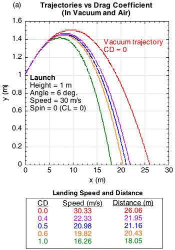
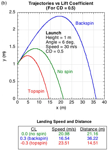
Figure 1 — Trajectories in a vacuum and in air — (a) results of altering the drag coefficient (CD) for identical launch conditions and no spin (CL = 0) — CD is typically about 0.5-0.6, so the trajectory doesn't depend very much on CD in practice; (b) results of altering the lift coefficient (CL) for the same initial launch conditions and the CD = 0.5 — CL is varied by varying the ball spin.
In the absence of all forces, a tennis ball will fly forever in a straight line at its launch speed, spin and angle. But no such absence exists and gravity pulls tennis balls down onto the court. If this were the only force (as in a vacuum), the trajectory would trace a perfect parabola. But, as Figure 1 shows, the presence of air introduces additional forces that alter the trajectory, namely the drag force and, for spinning balls, the lift force (aka the Magnus force). The drag force always acts opposite the direction of the ball's velocity and the lift force acts perpendicular to both the drag force and the spin axis. Lift force is somewhat of a misnomer since its direction can either be up, down or sideways (if the spin is sidespin) depending on spin. It is interesting to note that most research concentrates on CD and not CL. But it is evident from Figure 1 that even small changes in CL affect both speed and distance more than changing CD.
Figure 2 shows how drag, lift and gravitational forces combine to determine the shape of a trajectory.
Figure 2 — Forces acting on a tennis ball in flight: (a)Drag, lift and gravity forces during ascent and descent for topspin and backspin shots.
The drag and lift forces can each be separated into vertical and horizontal components, as shown in Figure 3. Though we tend to think of drag as acting only backwards and lift as up or down, we can see that each force can contribute to acceleration in almost any direction.
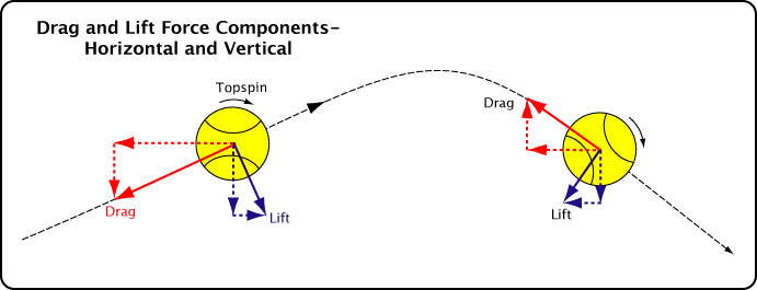
Figure 3 — Horizontal and vertical components of drag and lift forces for a topspin shot.
In reality, there is only one net aerodynamic force. It is the vector summation of the the drag and lift forces, or comparably, the summation of all the aforementioned components. Figure 4 displays the net aerodynamic force.
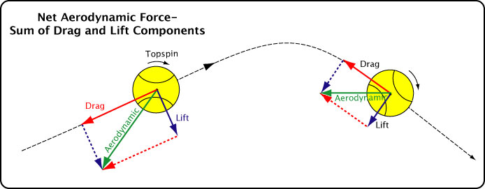
Figure 4 — Net aerodynamic force acting on a topspin shot in flight. The net aerodynamic force is equal to the vector sum of the drag and lift forces.
And finally, the total net force acting on a ball in flight combines gravity and the net aerodynamic force (Figure 5).
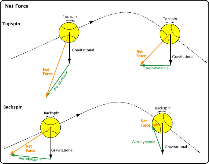
Figure 5 — Net of all forces acting on a tennis ball in flight. The total net force is equal to the vector sum of gravity, drag and lift forces. Both topspin and backspin shots are shown.
Given the evidence from Figures 1-5 that the magnitude of the drag and lift forces and coefficients make such a significant difference, it is essential to determine the magnitude and behavior of these coefficients that so significantly influence the trajectory.
II. THE EXPERIMENT
1. THE SETUP
The experiment setup was similar to one used by Kensrud and Smith [8, 9] for measuring the drag and lift force for baseballs, softballs, and cricket balls, except their experiment used light gates instead of video to measure speed and heights at two positions. The present experiment was performed in an indoors patio corridor with three brick walls and one glass wall. Cross hairs were drawn at two locations on the back wall and front glass wall, all at the same height. Camera 1 and camera 2 were arranged at the same height as the cross hairs. The camera 1 line of sight was about 0.5 m in front of the ball launcher and camera 2 was 6.4 m down range from that. When the front and back cross hairs were aligned in the middle of each camera's view finder, the cameras were then at the same height. A grid was drawn on the end wall and filmed by camera 3 to measure out-of-plane (z-axis) movement. Figure 6 shows the basic setup.
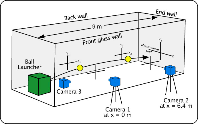
Figure 6 — Experiment setup.
Balls were launched at speeds from 14-30 m/s and spins between -2400 and 2500 rpm by a Tennis Tutor ball machine. Cameras 1 and 2 operated at 300 fps, 1/5000 s shutter speed, 150 mm zoom and with about a 80 cm x 60 cm view of the trajectory. A high zoom was necessary to see the ball in enough detail to accurately define its edges. Given such a small view window, the launch angle was altered after each change in spin or speed so that the trajectory would pass through each camera's view finder. Camera 3 was zoomed to 139 mm, shutter speed between 1/250 to 1/2000, and frames per second was 120. Six 500 Watt halogen lights were positioned between cameras 1 and 2 to illuminate the ball.
More experimental details are given in the Appendix: Seeing Should Not Be Believing: Calibrations, Distortions, and Errors.
2. THE BALL
The distinguishing feature of a tennis ball is its filament surface that manifests as "fuzz" to the player. This fuzz dramatically alters the flight of the ball, especially compared to a smooth rubber ball. We used Penn ATP Extra Duty balls for all shots, as shown in Figure 7. The average mass of the balls was 58.03 g and the average diameter was 65.68 mm. All balls were marked with perpendicular equatorial lines to determine spin (not shown in Figure 7). Balls were fed into the machine in a manner to launch the balls with the spin axis parallel to the camera's sight line (perpendicular to the plane of motion). Balls were fired in groups of 6 and repeated 2-4 times to make sure enough good, measurable shots were obtained.
Figure 7 — Ball used in experiment.
III. RESULTS
Aerodynamic results for balls are generally presented in two ways — CD vs Reynold's number (Re) and CD and CL vs Spin ratio (S) where
(4) Re = vD / k
where v is the ball's translational velocity, D is the diameter, and k is the kinematic viscosity of air at 20° C = 0.000015 m2/s,
and
(5) S = rω / v
where r is the ball radius, ω the rotational velocity in rad/s, rω is the tangental velocity at any point on the periphery, and v is the translational velocity.
Both parameters are non-dimensional and facilitate comparisons between different sized balls (for Re) and for balls with different spins and velocities (for S). Balls at the same Re have identical air flow characteristics around the object. From the Re equation (Equation 4), two balls, one with twice the diameter as the other, will have the same Re if the larger ball also travels at half the velocity. Similarly, any combination of spin and speed that results in the same S ratio will have similar rotational air flow. The Re and S results are shown in Figure 8. The spins and velocities are measured at x=0 of camera 1. All spins, S ratios, and CL have been made positive. The numbers in the Legend tables are the average values for each group of shots at a particular ball machine spin/speed setting.
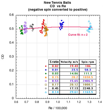
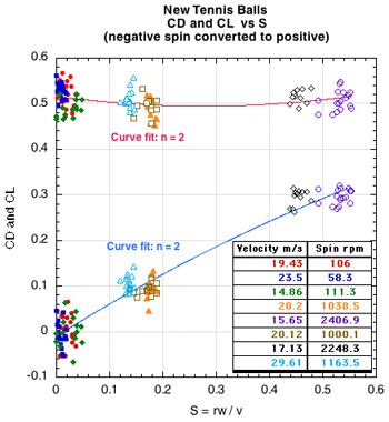
Figure 8 — Measured results of CD vs Re (left) CD and CL vs the spin parameter S = Rω/v (right) for new tennis balls. Note that if Re / 100,000 = 1.2 then Re = 120,000. The data in each graph is for all shots, spinning and non-spinning.
One hundred twenty-eight shots were measured for the new tennis balls. The velocity range was 14 m/s to 30 m/s and the spin range was -2400 rpm (backspin) to 2500 rpm (topspin); the range of CD was 0.453 to 0.567. The mean CD was 0.507 with a standard deviation of 0.024 and did not vary significantly with velocity or spin, however, there was significant shot-to-shot variation within any one group of shots at each ball machine wheel setting. CL varied almost linearly with spin parameter S, though, as with CD, there was significant shot-to-shot variation within each group and there was also significant lift even at very low spins. These variations are due to asymmetric fuzz orientation as explained in the Discussion section. The red and blue lines are quadratic best fits to the CD and CL data points.
Reynolds number is proportional to velocity when a single type of ball is being studied, but it is the universal method of comparing balls of different sizes. For reference, Table 2 shows the velocity in both m/s and mph for several Reynolds numbers.
| Table 2 Reynolds Number Conversions | ||
| Reynolds Number (Re) | Velocity (m/s) | Velocity (mph) |
|---|---|---|
| 50000 | 11.9 | 26.6 |
| 75000 | 17.8 | 39.9 |
| 100000 | 23.8 | 53.2 |
| 125000 | 29.7 | 66.4 |
| 150000 | 35.6 | 79.7 |
| 200000 | 47.5 | 106.3 |
| 500000 | 118.8 | 265.7 |
Table 2 — Reynolds number conversions.
IV. DISCUSSION AND ANALYSIS
1. AIR FLOW.
The drag and lift coefficients are the result of the type of air flow around the ball. Different ball types create different air flow. Furthermore, the results of this study suggest that different methods of testing also create different air flows. The average CD and CL in this experiment were significantly lower than the traditional wind tunnel results using a support sting (as were similar tests for shaved tennis balls and smooth balls, though the details of those results are not reported in this paper). However, wind tunnel experiments that dropped a ball through a wind stream had very similar CD and CL results to those presented here. Figure 9 shows some of these comparisons between ball types and testing methods: a generalized theoretical plot of CD vs Re (a), typical experimental results for several non-spinning ball types (b), and free-flight compared to wind tunnel results for CD (c) and CL (d).
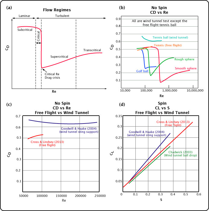
Figure 9 — Comparison of ball types and testing methods. The CD of the free-flight trajectory is considerably less than those for wind tunnels at the same Re. Similarly, this experiment measured smaller CL for given S for sting supported wind tunnel studies and similar CL for ball drop wind tunnel experiments.
(Based on Metha 2008 [10] and Goodwill, Chin & Haake [6]).
The terminology in Figure 9a refers to the "stages" of flow at various Re numbers. The "critical" stage is when the air flow changes from laminar flow to turbulent flow. Turbulent flow stays attached to the ball further along the surface and thus creates a smaller wake with less drag. As a result, the CD declines a significant amount if air flow achieves this transition due to sufficient speed and surface roughness. In the supercritical region, even though the flow is turbulent, there is a bit more friction drag due to the greater distance of attachment of the flow so the CD starts increasing. Further, the surface layer progressively thickens and begins to separate from the ball earlier and earlier as speed increases. Finally, in the transcritical regime, the CD reaches its maximum CD for turbulent flow, and it remains relatively constant for all higher velocities.
In brief, the factors determining the stages of air flow are listed below:
- Factors Influencing Air Flow
-
- A large wake indicates a large drag force and a narrow wake a lesser force.
- A downward directed wake is associated with an upward lift force, and an upward directed wake accompanies a downward lift force — as the ball pushes the wake air up or down, the wake pushes oppositely back on the ball.
- Wakes are diverted due to spin and surface asymmetries on opposite sides of the ball, due to design (seams on a baseball), wear, surface deformation during flight (tennis ball fuzz), etc.
- The characteristics and behavior of the boundary layer (the layer of air closest to the ball's surface) determine wake behavior. A turbulent boundary layer stays on the ball for a longer distance before separation and wake formation, thus forming a smaller wake. A laminar boundary layer separates earlier, resulting in a larger wake.
- Ball shape and surface topography determine boundary flow: rough surfaces (like raised seams or fuzz) create turbulence and smooth surfaces promote laminar flow.
- Drag force increases with velocity, but at a characteristic velocity for each ball (the "critical" velocity), the drag force and drag coefficient suddenly decrease, sometimes by as much as half or more. This is known as the drag crisis.
- The drag crisis occurs when air flow transitions from laminar to turbulent flow.
- Spin causes one side of the ball to be moving faster than the other with respect to the surrounding air, influencing transition points and boundary layer thickness. Thus, boundary layer separation will occur at different locations on the top and bottom of the ball, diverting the wake in a direction depending on the spin direction. Surface variances on opposite sides of the ball can cause the same asymmetric separation.
- Tennis balls do not exhibit a drag crisis at any previously tested velocities because the fuzz causes the boundary layer to be turbulent at all velocities common to tennis play.
- Essentially, the CD and CL are multipliers for the effect of all these surface phenomena.
Figure 10 displays these relationships.
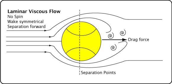
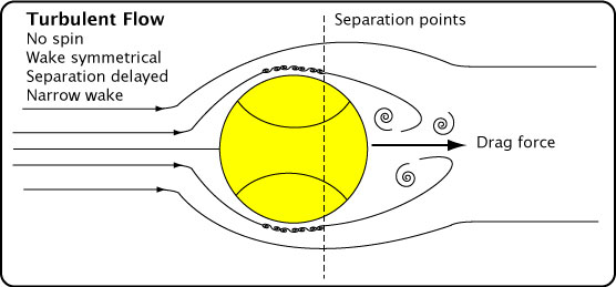
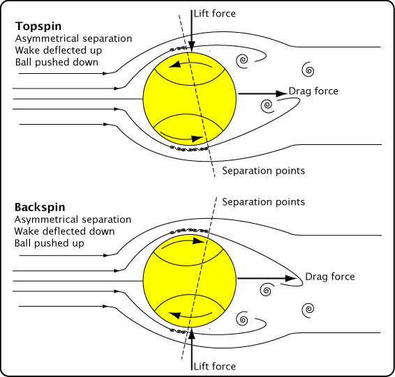
Figure 10 — Types of air flow on tennis ball. Laminar, turbulent, and spinning. In the drawings, the ball is stationary and the air flow is from the left. If, instead, the air is stationary and ball travels to the left, then the drag force remains as indicated — to the right.
Flow type is also determined by the influences of surface friction between the air and the ball and the viscosity of air. Viscosity is a measure of how a fluid flows. It is a measure of the stickiness of adjacent layers of fluid to each other when one layer is subjected to a shearing force (caused by the ball). As the air flows, the layer next to the ball actually sticks to the ball (the "no slip" condition characteristic of all interactions between a fluid and surface of an object). The relative velocity of the ball to air is zero for this layer. Layers further away from the ball's surface are slowed by the layer below it, but each less so. Each layer up from the surface has a higher relative velocity to the ball until a layer is reached that is no longer influenced by the frictional and viscous effects caused by the ball (known as the free stream flow). Figure 11 shows this "velocity gradient" of air layers.
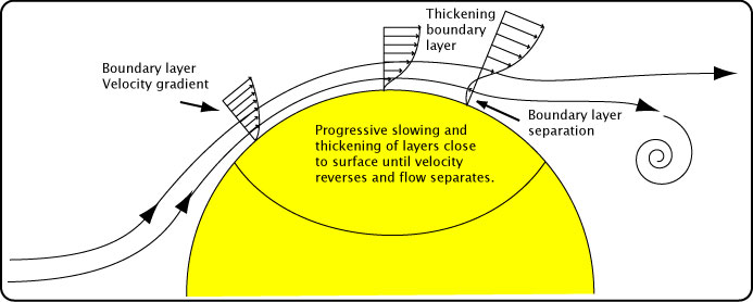
Figure 11 — Boundary layer velocity gradient.
Taken together, this area of velocity gradient is known as the boundary layer. As the boundary layer develops from the front to back of the ball, it grows thicker and effectively changes the shape of the ball because the free stream flow behaves as if the edge of the boundary layer were the surface of the ball. At first, the boundary layer development is an orderly progression and the sub-layers do not mix together. As the flow progresses over the ball, flow becomes unstable and very small disturbances, fluctuations, and mixing begin to occur. At higher speeds this creates a transition point where flow changes from laminar to turbulent. When flow becomes turbulent, the boundary layer next to the ball gains more energy and momentum as faster sub-layers of air above mix with the slower sub-layers below, enabling the boundary layer to overcome the adverse pressure gradient that exists from the apex of the ball toward the back. This extra momentum allows the boundary layer to stay attached to the ball for a longer distance before it peels away.
The lower CD results of this experiment compared to wind tunnel experiments indicate that the flow separation is delayed on free flight trajectories compared to wind tunnel simulations, creating a smaller wake and less drag. The lower CL indicates that there is less asymmetric wake diversion than indicated by the wind tunnel.
2. THE FUZZ EFFECT
The fuzzy filament surface is primarily responsible for the turbulent flow around a tennis ball at all speeds of interest. Because the transition from laminar to turbulent flow occurs at all usual playing speeds, tennis balls do not exhibit a drag crisis during games. However, as air flows through the filaments, each filament contributes its own drag force to the total drag force on the ball. That is why the CD for a tennis ball is higher than all other balls at all speeds shown in Figure 9b, even though it is in the super-critical flow regime throughout its flight where CD is typically lower than at its precritical speed. The fuzz topography is constantly being reconfigured due to collisions with the racquet and court and due to its flight through the air. It is hypothesized that it is the changing fuzz configurations that are responsible for the significant shot-to-shot variations in CD, even at the same ball machine wheel settings. The changing fuzz landscape causes variations in effective ball diameter, the rate and amount of turbulent boundary layer thickening, and the location of the turbulent transition point. Together, these effects will influence the boundary layer separation points and thus the size and direction of the wake.
Consequently, we wanted to take a closer look at ball fuzz and see if we could capture its movement and orientation in flight. To do so, we backlit the trajectory paths, revealing a fuzz length that is quite amazing and only becomes apparent with back lighting and fast image capture. Players see a perfectly smooth ball, partly because the eye can't capture the image fast enough. The eyes just see an average edge. Balls were shot at about 50 mph and filmed at 300 fps. Figure 12 demonstrates how spin alone affects the ball's fuzz surface. Balls are moving left to right. Topspin rotation is clockwise and backspin counter-clockwise.
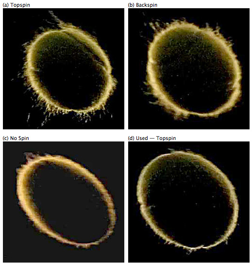
Figure 12 — Mid-flight fuzz alignment for shots with new balls of topspin, backspin, no spin and an a used ball with topspin.
In general, Figure 12 shows that fuzz lays down when it is spinning toward the oncoming air (top of ball in topspin and bottom in backspin) and it stands up when it is spinning away from the air (bottom of ball in topspin and top in backspin). The fuzz on a non-spinning ball lies down on both the top and bottom of the ball and there is very little fuzz on a used ball. However, tufts of fuzz can dislodge, standup, or otherwise protrude into the airflow, even on the forward moving side of the ball, as seen on the top of the ball in Figure 12a. It is this type of random fuzziness that can make the CD and CL vary for shots of identical speed and spin.
(Note: The slightly elliptical ball shapes are camera distortions. In these photos, the camera shutter is exposing light from top to bottom and the ball is moving rapidly left to right. Even though the shutter speed was 1/5000 second, by the time the bottom of the ball was exposed, the ball had moved to the right, so in effect, top and bottom were shot at slightly different locations, stretching the ball's appearance (see more examples in Appendix: Rolling Shutter and Zoom Distortion).
Movie Screen 1 shows an exaggerated simulation of the fuzz effect for topspin and no spin. Notice how the "fuzz" on antipodal sides of the topspin ball orient in opposite directions, whereas it is more symmetrical with no spin. The wind is blowing from right to left in these movies.
Movie Screen 1 — Exaggerated fuzz effect simulation for topspin and no spin.
Note on movies: It is easier to see the fuzz transitions by advancing one frame at a time using the right or left arrows on the keyboard or movie progress bar.
It is evident from watching this simulation in slow motion that the stiffness, quantity, density and length of the fuzz fibers will influence the standup/sit-down effect on the oncoming and retreating sides of the ball. This in turn will influence the CD and CL. Further, as the ball rotates, it continuously presents new profiles to the oncoming air. Therefore, it is the average of the advancing and retreating side profiles over a trajectory that will influence the CD and CL. This is illustrated in the following sequence of a topspin shot (Figure 13), each frame separated by 0.003 seconds and about 1/9 revolution (about 2000 rpm).
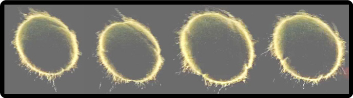
Figure 13 — Changing aerodynamic profile. As the ball rotates, a new fuzz profile is presented to the oncoming air. (The frames with slightly larger balls are due to photo cropping, not expanding balls.)
The profile of the fuzz filaments in the sequence of Figure 13 are remarkably like those of the simulated fuzz in Movie Screen 1. The fuzz tries to lie down on the advancing side, gets squashed in the front, and tends to stand on the retreating side.
3. CD, SPEED AND SPIN
Figure 14 shows the behavior of CD with and without spin with changes in Re and comparisons of those results with a typical wind tunnel result. We wanted to compare free flight and wind tunnel findings on two fronts: the behavior of CD at low Re without spin and at constant speed with increasing spin. Previous wind tunnel findings indicated that CD increased at low Re and with increasing spin. The first comparison was straight-forward, the second a bit complicated.
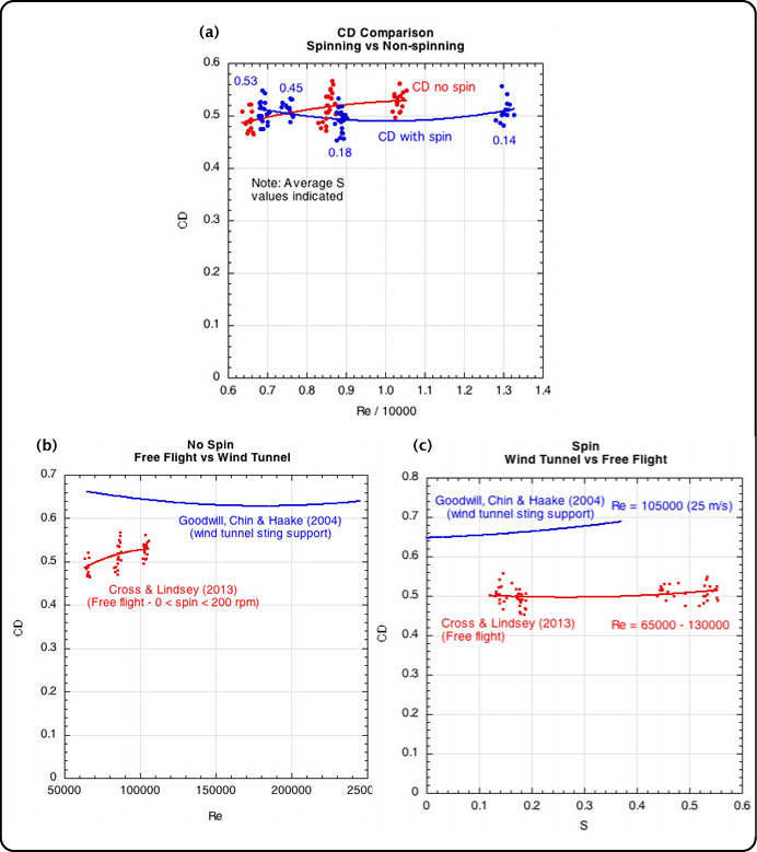
Figure 14 — CD with and without spin with comparisons to typical wind tunnel results.
First, Figure 14 shows that the free-flight CD decreases at very low Re (< 100,000) for a ball with no spin (< 200 rpm). This is the opposite of most wind tunnel studies that show that CD increases at lower Re (lower speeds), as illustrated in the Figure 14b. Both curves level out at higher Re. At lower speeds, the fuzz tends to stand up more and then progressively lies down as wind speed is increased. When the fuzz stands up it will effectively increase the diameter of the ball and allow air to flow through the filaments, both of which create more drag. This is a sound argument. Why then did the CD decrease at low Re in the free flight experiment?
A possible mechanism for the decrease in CD at low Re is described in Chadwick [11] and is known as the Brown effect. Brown proposed to slow the game of tennis by adding nodules to the ball. He showed that the CD decreased at lower Re (below playing speeds) because the nodules tripped an early transition to turbulent flow and that the air flowed through and around the nodules, so they did not increase effective diameter as much as expected and CD remained lower. However, as Re increases, the air flowed over the nodules and thus increased the effective diameter and widened the wake, increasing the CD.
The same effect applies to a regular tennis ball. At low Re, the fuzz is more upright and the air flows through the fibers. In doing so the surface friction increases which will delay boundary layer separation. As the air speed increases, the filaments begin to lie down. They do not lie flat, however. As each filament leans over, it is constrained by the filaments immediately behind it. As this process progresses over the surface of the ball, it is like dominoes falling on each other, such that the fuzz becomes compacted and forms a fuzz ramp as you move toward the apex of the ball. As air streams over the ball, it no longer flows through the fibers and it is forced up the ramp and separates from the ball. This creates a larger wake region and higher CD. This process continues until an Re is attained where compaction and ramping reaches a limit and CD remains relatively constant as Re continues to increase. The result is a CD curve that looks more like the expected supercritical behavior as seen in Figure 9c. Figure 15 illustrates this effect.
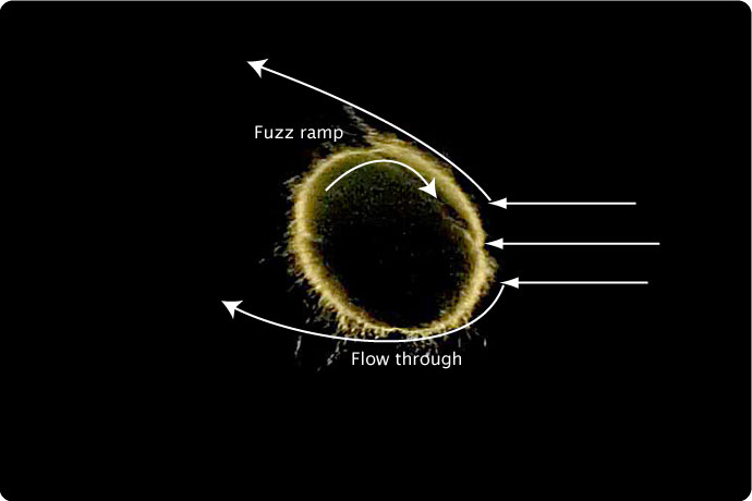
Figure 15 — Effect of filament lie-down, compaction, and ramping on CD. At low speeds the air flows through the filaments. At higher speeds the fibers form a ramp that facilitates boundary layer separation.
Secondly, it would appear from Figure 14a that shots with spin have a lower CD than those without spin, except as S increases above about 0.4. This too would be contrary to wind tunnel findings. However, Figure 14c indicates that if the ball is spinning, the CD increases slightly for both wind tunnel and free flight balls as S increases. The two methods agree on this. But why would the spinning ball have a lower CD than a non-spinning ball? The fuzz ramp effect explanation would seem to be relevant here too.
At low speeds the fuzz on the top and bottom of the ball will be standing and there will be no fuzz ramps. As speed increases, a ramp will form on each side. On a spinning ball at low speeds, the advancing side of the ball may have a ramp and the retreating side may be more upright. If that is the case, we can explain the two curve fits in Figure 14a. At Re around 70000, the non-spinning ball has two ramp-free surfaces and the high spin, high S, ball might have a fuzz ramp on the advancing side and not on the retreating side. At this Re, the spinning ball has a higher CD. As Re increases, the non-spinning ball starts the formation of ramps on both sides, whereas the spinning ball still has one side with and without a ramp. So, depending on the Re and S, a spinning ball will have a lower CD than a non-spinning one. But as Re increases, both sides of both will have ramps, and the difference in CD will flatten and tend toward constancy.
The ramp effect would have to be stronger than the competing effect of more fuzz drag when the fibers are standing up. Air flowing through the fibers must cause a later separation point than the increased fuzz drag due to that flow through.
The explanation here is somewhat speculative. It may indeed be correct, but further experiments would be needed to investigate the phenomena in more detail. For example, a study could be be undertaken using smooth balls with different amounts and different patterns of added fuzz. Beyond that, even if it is correct, why do the two test methods arrive at different results for CD at low Re? Even if the explanation for each behavior makes sense, why are we seeing two different behaviors needing separate explanations?
V. CONCLUSION
It would seem that there is some inherent difference between the free flight and wind tunnel methods of testing for CD and CL. Not only were significant quantitative differences found, but there were also qualitative differences. Both the magnitude and behavior of the coefficients differed between the methods as Re and S varied.
First, a difference in the magnitude of measured drag and lift coefficients between free flight and wind tunnel experiments was observed. The CD and CL were both significantly lower than traditional sting support wind tunnel measurements, but they were similar to ball drop wind tunnel tests. Lower values for these coefficients implies lower drag and lift forces with an attendant less slowing, diving or floating of the ball than wind tunnel values would predict.
Second, the CD did not show the same increase at lower Re as do the usual wind tunnel studies. In fact it decreased at lower Re. This is more in keeping with the theoretical shape of the CD curve in the supercritical and transcritical regimes but at odds with the accepted explanation of the behavior and effects of fuzz on air flow at lower Re. Another mechanism is offered here to explain the low CD findings — the "fuzz ramp" effect. This explanation is speculative at this point, and even if true, it still doesn't explain why the two methods observe such different behavior to begin with.
Third, both free flight and wind tunnel experiments show CD to increase with spin. However, the free-flight experiment also showed the CD to be lower for spinning balls compared to non-spinning balls. It was hypothesized that this occurs because non-spinning balls can develop two-sided fuzz ramps at low but increasing Re, and spinning balls, up to some limiting Re, may only have one ramp. This results in lower CD for the spinning ball. At very low Re, the wind speed is not sufficient to create fuzz ramps on a non-spinning ball, and the air flows through the fibers instead. This delays boundary layer separation and lowers CD compared to the spinning ball.
Fourth, perhaps the biggest surprise finding of the experiment was the significant shot-to-shot variance in CD and CL. This is the result of significant alterations in air flow due to seemingly small variances in the fuzz profile presented to the oncoming air, including ever changing fuzz ramps and flow-through scenarios, as described in the Discussion section.
This study perhaps raises more questions than it answers. Because it is the first true free-flight study of its kind (at least, known to the authors), repeatability of its results by others is needed for confirmation. Also, it would be fruitful for further study to have a ball launching machine that could achieve higher speeds and could independently vary the speed and spin of the ball.
Free flight study is inherently problematic due to the difficulty in accurately pin-pointing position during flight. This difficulty is magnified as the length of the trajectory increases. This study took every precaution possible to minimize this uncertainty, as described below in the Appendix.
VI. APPENDIX:
SEEING SHOULD NOT BE BELIEVING: CALIBRATIONS, DISTORTIONS, AND ERRORS
The most essential thing is to accurately measure both the position and the speed of the ball. The change in horizontal speed determines CD and the change in vertical position determines CL. We used two positions, one near x = 0 to measure speed at camera 1 and one at x = 6.4 m to measure at camera 2. The change in the x and y coordinates between the two camera positions is the starting point for all calculations. Drag and lift coefficients are very sensitive to small errors in position measurement. Error can creep into the experiment in many unseen and unexpected ways and it all adds up. The goal was to measure position to an accuracy of 1% or better. This is especially necessary when the experiment yields results that differ from previous experiments. How do you know whether your findings are real or not? We discuss several potential error sources and how to identify or prevent them below.
1. Standardize Reference and Camera Heights. As discussed in the setup, great care was taken to make sure the cameras were at the same height and tilt and focused in the same plane. The basic problem is this: suppose the ball follows an arc, starting and ending level with a horizontal line on the back wall. How will we know if it indeed does so? Camera 1 might look down onto the line and camera 2 might look up. Camera 2 will say the ball passed under the line. Camera 1 will say the ball passed over the line. So both cameras need to be at the same height and zoomed to the same distance.
One might think all that is needed is a meter stick, T-square or laser level to accomplish a perfectly horizontal line on the back wall. But what if the floor slopes, or the laser is 0.1 degree off? Over 8 meters, a 0.1 degree error in laser level balance can lead to 14 mm error at the other end. We chose to let fluid pressure do the measuring for us by using a water level to draw the horizontal line, as shown in Figure 16. We did the same for the cross-hairs on the glass walls and then, as a check, between the back wall and the glass doors.
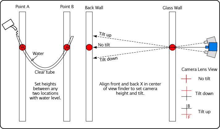
Figure 16 — Measuring equal heights. First you measure your desired height at point A and mark it. Pour water into the clear tube, making sure there are no kinks or bubbles in the tube. Move the tube up and down at point B until the height of the water at point A is exactly at the desired height. Mark your spot at point B. This method is essentially a U-tube manometer that operates on the principle that the pressure on a liquid at equal heights is the same at each location. To align each camera to that height, raise or lower the camera until the cross-hairs on the front and back walls line up in the center of the view finder in the "no tilt" position shown on the right. If the camera is too high, the front cross-hair will appear below the back, and vice versa if it is too low. You will also have to move the camera right or left to make the verticals line up.
2. Calibrate Distance and Out-of-Plane Correction Factor. The most essential part of the experiment is to calibrate the distance scale. To do that, at each camera we filmed an object of known length in the plane of the desired trajectory (Figure 17). When viewed through the view finder, that same object appears smaller when moved backward and larger when moved forward. If the object is 60 cm long, as was our calibration board, then when moved backwards it might appear as 58 cm compared to the 60 cm board, and when moved forward, it might appear as 62 cm. The apparent size will vary with distance backward and forward. The same thing will happen with the ball and the measured distances of travel when the trajectory is forward or backward of the calibration plane. If the ball travels in front of the calibration plane, distances will measure longer, speeds higher, and drag and lift coefficients will calculate as less than they really were between the two cameras. The opposite would occur if the ball were behind the calibration plane. We need a method to correct for this difference between the seen distance and actual distance.
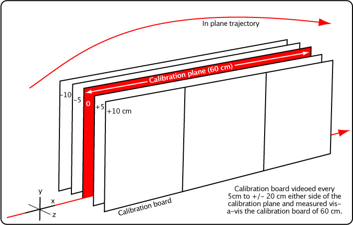
Figure 17 — Distance calibrating of the camera.
To do so, we filmed the calibration board in several positions forward and backward of the calibration plane, as shown in Figure 17. We plotted the "seen" length vs the position forward or backward. We fit a second order polynomial to the plot points. The equation for the polynomial thus tells you what the seen length will be for any z-axis (toward or away from the camera) amount. The ratio of the calibration length to the seen length gives the correction factor for distance calculations. For example, if you measured the diameter of the ball and it was 67.3 mm, and if the correction ratio were 0.98 (meaning the ball must have been in front of the calibration plane), then the corrected diameter would be d = 0.98 x 67.3 = 66 mm. Figure 18 shows the calculations for this experimental setup.
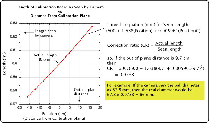
Figure 18 — Calculating the calibration correction ratio.
Now we know how to correct for a ball that travels in front or behind the calibration plane, but how do we know whether or how much it was out of plane (e.g., the 9.7 we used in Figure 18)? Camera 3 is setup to capture the out-of-plane variance at impact on the back wall. But what we really want to know is the variance at the camera 2 position at 6.9 m from the ball launcher (the launcher is 0.5 m before the x = 0 position of camera 1). Figure 19 shows the geometry to determine this. Triangles abc and ade are similar triangles so the ratio of their sides is the same. So, ad/ae = de/bc = z/x. Solving for z gives the out-of-plane distance at camera 2.
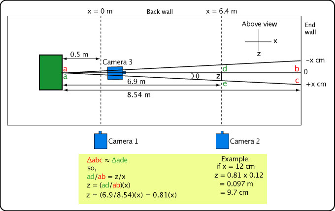
Figure 19 — Calculating the out-of-plane distance at camera 2.
3. Perspective/Parallax Error. As explained above, an object changes its perceived location and size as it moves perpendicular to the plane of the video. This in turn will affect the measured velocities. We corrected for this with the out-of-plane calculation above. However, there's another aspect of this perspective problem that will affect the perceived location of the ball. Because the ball is a three-dimensional object, there is always part of it that is in front of the calibrated plane of motion and part of it behind. All of our calculations are based on the center of the ball. Depending on the shape and size of the object, its distance from the camera, and its angle from the camera's perpendicular view of the plane of motion, there can be a discrepancy between the perceived and actual edge and center locations that you are trying to measure. Figure 20 illustrates how the 3-D ball distorts perception.
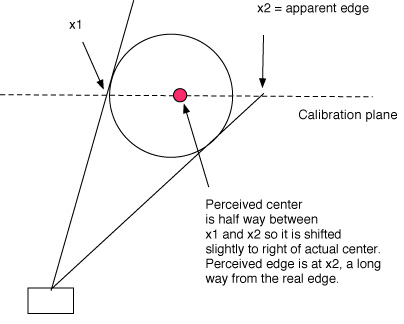
Figure 20 — Perspective error. Perceived vs actual location.
For this experiment, the cameras were 3 meters from the trajectory plane. The ball was measured over a distance of about 60 cm, 30 cm on each side of the center of view. That means that the greatest the angle was from perpendicular during measurement was about 0.15° (arcsin(0.03/11) = 0.15). That should not make much of a difference in our measurements, but we tested to make sure.
We did the following experiment to check for parallax error. First the video plane was calibrated. Balls were set up on a table in the plane of calibration. A paper measurement grid was placed on the table under the balls. An engineer's square was used to place the outside edge of the ball directly at 10 cm intervals. The edge as presented in the video was measured from the center of view in motion analysis software, and then compared to the actual measurement. Figure 21 shows the setup.
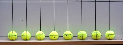
Figure 21 — Parallax test setup.
The result was that for the 3 m camera distance from the ball and the 70 cm left-right viewing range, the measured edge and actual edge were virtually identical and no correction was necessary.
4. Check for Camera Lens Distortion. Camera lens distortion can lead to measurement errors. The errors are usually greatest at the periphery of the image. For that reason, if there is known distortion, it is best to limit measurements to the center of the image and to zoom in, which narrows the view to the center. Common types of distortion are the barrel and pincushion distortions. As shown in Figure 22, these distortions can under-estimate distance and velocity (barrel) or over-estimate them (pincushion).
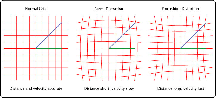
Figure 22 — Common types of lens distortion. The effect on distance and velocity measurements of barrel and pincushion lens distortion. The same blue diagonal line and green horizontal line are transported from the normal to barrel and pincushion grids. The barrel distortion grid measures those lines as short and the pincushion grid sees the same lines as long, according the respective measurement grids. Different parts of the distortion grids decrease or increase the effect more than others as seen the apparent length difference of the red and green lines in each of the grids.
Figure 23 shows one method to check for lens distortion. A grid of 1-centimeter squares is taped to a wall and filmed at various zoom levels. As zoom increases, the view angle of the grid decreases. Figure 22 is the grid as seen at zoom = 93 mm. The camera was 520 mm away from the grid.
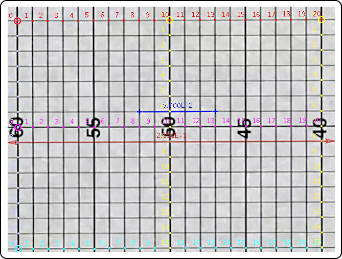
Figure 23 — Technique for checking for camera lens distortion.
With the help of motion analysis software, the periphery and the center of the grid were digitized. Five horizontal and five vertical points were selected at each of 9 locations (top left, middle and right; middle left, middle, and right; and bottom left, middle, and right). These points were digitized on successive frames of the movie, so each point 1-centimeter point was separated by 0.00333 seconds (filmed at 300fps). The 5 cm blue line is the calibration reference. All measurements between points on the grid and calculations based on them are in relation to that fixed distance. At any of these 9 locations, a horizontal or vertical 5-box section should be 5 cm long if there is no distortion (though there will be some digitizing error). Figure 24 shows the percentage distortion for each horizontal and vertical 5 cm segment at each location and at several zoom levels.
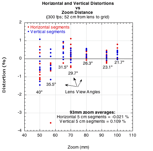
Figure 24 — Percentage of camera lens distortion at 9 locations and two directions in the camera view.
As zoom increases, distortion decreases. For the grid shown at zoom of 93 mm shown in Figure 23, the average distortion for rows was only 0.21% and for columns, 0.109%. The trajectory experiment was filmed at a zoom of 150 mm, so distortion was presumably even less. At a zoom of 50 mm, the distortion was greater than 1.0 % in some locations.
5. Rolling Shutter and Zoom Distortion. As explained above in the Fuzz Effect section, the camera shutter is exposing light from top to bottom and the ball is moving rapidly left to right. Even though the shutter speed was 1/5000 second, by the time the bottom of the ball was exposed, the ball had moved to the right, so in effect, top and bottom were shot at slightly different locations, stretching the ball's appearance. To make matters worse, even though a higher zoom minimizes lens distortion, it increases the rolling shutter distortion. Figure 25 shows an example of balls traveling about 19 m/s (43 mph).
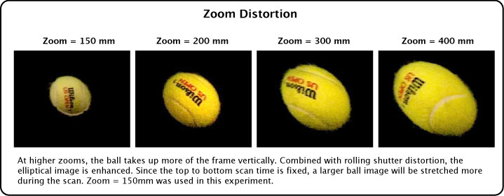
Figure 25 — Rolling Shutter and Zoom distortion. Combined with rolling shutter distortion, increasing the camera zoom will increase the elliptical distortion.
This experiment was filmed at zoom of 150 mm. There is little distortion at this zoom, but it is still apparent and could affect methods to accurately digitize the center of mass of the ball. Special methods were therefore developed to locate the center of the ball in each frame, as discussed below.
6. Digitizing Methods. Further complicating our efforts to locate the center of mass is that sometimes the edges of the ball were blurry, poorly lighted, against a non-contrasting background, or the ball elliptically deformed. To account for these difficulties, each author digitized the ball center at x=0 and x=6.4 m separately using different methods. The average of the two methods was taken as the position, and the difference in the x and y coordinates divided by 2 was taken as the digitizing error. The most comprehensive of these methods is shown in Figure 26.
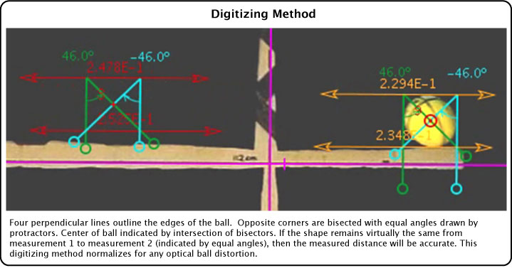
Figure 26 — Digitizing method to normalize for optical ball distortions and edge uncertainty.
At each camera location, the ball speed is calculated from the two ball centers located by the above procedure. The measurement points were an equal number of video frames to either side of the y-axis. The centers were typically about 400 mm apart horizontally and about 40 mm vertically. Consequently, the same magnitude error in the x or y position results in a larger percentage error possibility in the y direction compared to the x direction.
7. Camera Frame Rate Error. If the camera is filming at other than the indicated 300 frames per second, then our measurements of speed and spin would not be accurate. To verify the frame rate, we filmed both digital and analog watches for 10 seconds (Figure 27). Ten seconds should be 3000 frames. The cameras filmed between 299.7 and 300.1 fps.
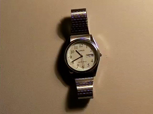
Figure 27 — Frames per second test. Filming a second hand at 300 fps for exactly 10 seconds should be 3000 frames.
References
1. Zayas J (1986) Experimental determination of the coefficient of drag of a tennis ball. Am J Phys 54(7):622-625.
2. Stepanek A (1988) The aerodynamics of tennis balls - the topspin lob. Am J Phys 56(2):138-142.
3. Chadwick S, Haake S (2000) The drag coefficient of tennis balls. In: Subic A, Haake S, eds. Engineering of Sport, Research, Development and Innovation: Proceedings of the 3rd International Conference on the Engineering of Sport; Sydney, Australia. Blackwell Science: Oxford; 169-176.
4. Chadwick S, Haake S (2000) The determination of the coefficient of drag of three different tennis balls using a wind tunnel.
5. Mehta R, Pallis J (2001) The aerodynamics of a tennis ball. Sports Engineering 4(4):113.
6. Goodwill S, Haake S (2004) Aerodynamics of tennis balls effect of wear. In: Hubbard M, Mehta RD, Pallis JM, eds. The Engineering of Sport 5: Proceedings of the 5th International Sports Engineering Association Conference. Springer: Hoboken, 2004; 35-41.
7. Goodwill S, Chin S, Haake S (2004) Aerodynamics of spinning and non-spinning tennis 15 balls. Journal of Wind Engineering and Industrial Aerodynamics 92:935-958.
7. Alam F, Subic A, Watkins S (2003) An Experimental Study on the Aerodynamic Drag of a Series of Tennis Balls. Proceedings of the Sports Dynamics-Discovery and Application: The International Congress on Sports Dynamics; 13 September 2003, Melbourne, Australia. 22.
8. Kensrud J, Smith L (2010) In situ drag measurements of sports balls. Procedia Engineering 2:2437-2442.
9. Kensrud J, Smith L (2011) In situ lift measurement of sports balls. Procedia Engineering 13:278-283 16.
10. Mehta, R (2008) Sports Ball Aerodynamics. Sport aerodynamics. In: Norstrud, H, ed. Sport Aerodynamics; SpringerWien, New York, 2008; 229-331.
11. Chadwick, S.G. (2003) The Aerodynamic Properties of Tennis Balls. Ph.D. Thesis, University of Sheffield, Sheffield, UK.
12. Brody H, Cross R, Lindsey C (2002) The Physics and Technology of Tennis. Racquet Tech Publishing, Solana Beach CA.
13. Cross R, Lindsey C (2005) Technical Tennis, Racquet Tech Publishing, Vista CA.