ABSTRACT
This study is of a pilot project to test the traction of tennis shoes. A test rig was built to study translational and rotational traction. Shoes were loaded vertically and horizontally at forces typical of actual tennis play. A court suface was prepared by Decoturf similar to that used for the U.S. Open. The translational tests were performed with the shoe aligned parallel to the direction of movement. For the rotational tests, there was no translation and all motion was around an axis at the ball of the foot. The purpose of the study was to ascertain the forces that are important to the generation of translational and rotational traction, independent of surface or shoe type. Forces generated by the test rig could then be calibrated to those measured in the field, and the results will then be used to determine relevant parameters for further testing and to develop a comparative footwear database of traction.
1. INTRODUCTION
Tennis footwear is essential to performance, comfort, and injury prevention. A tennis shoe must facilitate stopping, turning, and propulsion and do so on many surfaces under many conditions — grass/asphalt/clay/acrylic/carpet; dry/wet, hot/cold, clean/dirty, new/worn, rough/smooth, etc. While the shoe is performing all these tasks, it must do so without causing injury. Friction and stiffness are the two properties that are primarily involved. Friction is responsible for stopping, turning, pushing off, and sliding parallel to the court. Stiffness performs the jobs of shock absorption, deceleration, and energy return, mainly in the vertical direction.
Translational Traction. "Friction" and "traction" are often used interchangeably. However, in the context of footwear, the term "traction" is generally used. This highlights the propulsive nature of the motion [1]. Traction is also used to distinguish frictional interfaces with compliant surfaces as opposed to noncompliant ones [2]. The latter interactions obey the traditional Amontons-Coulomb laws of friction which state that friction is (1) independent of surface area, (2) directly proportional to normal load, and (3) independent of relative velocity of the surfaces. Instead, tractional interfaces between compliant surfaces disobey all these "laws" and are influenced by a number of factors: surface roughness, surface and shoe stiffness, normal force, contact area, pressure, loading rate, sliding rate, frictional induced torque, contaminants, wear, tread, shoe orientation, and temperature. These all affect the adhesional and/or hysteretic properties of the contact between the two surfaces. The adhesional properties depend on the atomic and molecular bonds formed at contact points (asperities) of the two surfaces. The strength of these bonds will depend on the difference between the real and apparent contact areas. With higher normal forces, lower velocities, and softer materials, the real contact area of asperities will increase. Hysteresis manifests itself due to the viscoelastic nature of the surfaces such that energy is consumed as the contact asperities deform due to shear forces [3, 4]. This prevents or retards the relative motion between the two surfaces. This is especially true when one surface is much softer than the other.
Coefficient of Traction. The usual method of comparing the translational traction of various shoe-surface interactions is by comparing the resulting coefficient of traction (COT). The coefficient of traction is a unitless ratio that indicates the resistance to sliding of two interacting surfaces that are being pressed together by a force. This is the ratio of the horizontal (traction) to the vertical (normal) reaction forces resulting from an applied shear force to the surfaces (Equation 1, Figure 1):
(1) COT = Ft / Fn or, Ft = COT x Fn
Where Ft is the instantaneous traction ground reaction force, Fn the normal or vertical ground reaction force, and COT is the coefficient of traction.
Up to some maximum, the traction force matches the applied horizontal force, keeping the surfaces from moving relative to each other. The maximum traction force that exists just before relative motion ensues gives the maximum coefficient of traction. This coefficient is referred to as the coefficient of static or available traction (COTA):
(2) COTA = Fp / Fn
Where COTA is the coefficient of available traction, Fp is the peak traction force and Fn is the normal force.
Once moving, the force necessary to keep the surfaces moving at constant velocity gives the coefficient of dynamic traction (COTd). The dynamic coefficient is generally less than the static coefficient. The minimum horizontal force to keep the sufaces moving at constant velocity is Fmin. The dynamic ratio that is usually listed as the COTd is thus:
(3) COTd = Fmin / Fn
Where COTd is the minimum coefficient of dynamic traction, Fmin is the minimum force necessary to keep the surfaces moving at a constant velocity and Fn is the normal force.
For example, if the COTA between a 100 lb box and the floor is 0.5, then a horizontal force of 50 pounds is required to initiate sliding of the box along the floor. If the COTA is 0.8, an 80 lb force is required, and if it is 1.2, then 120 lb is required. If the COTA of the 100 pound box is 0.8 and the dynamic COT is 0.6, then it takes an 80 lb horizontal force to start the box moving and a minimum of 60 lb force to keep it moving at a constant velocity.
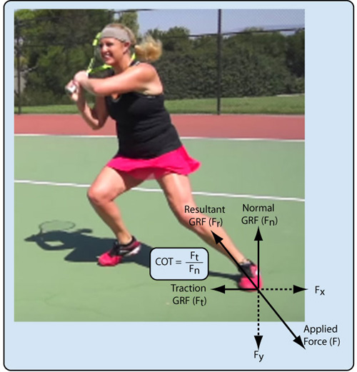
Figure 1 — Traction is necessary to both stop the player's motion after planting the lead foot and then to propel the player during and after the hit. Traction is created by frictional forces between the shoe and court. The force of the foot strike creates an equal and opposite ground reaction force (GRF) that can be split into a vertical and horizontal component. The vertical component is the normal ground reaction force and the horizontal is the traction ground reaction force. The coefficient of traction (COT) is the ratio of the two.
Rotational Traction. Whereas translational traction is measured with peak horizontal force, rotational traction is measured using peak moment of rotation (torque). The moment is calculated by multiplying the force times the perpendicular distance from the line of the force to the axis of rotation:
(4) τ = torque = F x r
where τ is torque (moment of rotation), F the shear force, and r the perpendicular distance from the line of force to the center of rotation. Peak force is used to calculate peak moment of rotation. The distance r (the moment arm) is the approximate distance from the turning axis in the forefoot to where the heel or ankle would be. For the size 9 men's shoe, that distance (r) was held constant at 120 mm.
Excessive traction during rotation has been associated with lower extremity injuries by many researchers. A shoe must simultaneously facilitate turning while simultaneously limiting translational slipping. The danger is that the shoe will become stuck to the surface and all the torque will get transferred to the ankle and knee joints.
Mechanical vs Player Traction Testing. Traction can be tested using mechanical test rigs or with players actually performing movements. Both techniques have advantages and disadvantages and both are necessary. Mechanical testing is controlled and repeatable. With mechanical testing, one variable at a time can be manipulated and controlled while keeping all others constant. The effect of that variable on traction can then be assessed and the mechanics of that effect might be determined. The disadvantage of mechanical testing is that the actual movements, forces, durations, and distances experienced by players are very difficult to simulate. Further, test rigs designed by different researchers all differ from each other, yield situation-specific results, and no test or method has been accepted as a tool for universal comparison of footwear traction. All that being said, what mechanical traction tests do best is to determine the maximum available traction from a specific shoe-surface interface at any given normal and shear-loading force. As mentioned above, this is the peak available traction force before sliding occurs and is quantified by the coefficient of available traction — COTA.
Player testing is more realistic but not entirely consistent, repeatable, or generalizable. One problem is that players must still perform semi-simulated moves and be instrumented. Players must plan their moves to land on force plates or enter a test area at certain speeds and they may be hooked up with reflectors or wires, all of which compromise the movements. Modern wireless pressure insoles are a promising technical advancement for studying foot-shoe-surface interactions.
Available Traction vs Utilized Traction. Mechanical traction tests are used to determine the maximum available traction from a specific shoe-surface interface at any given normal and shear-loading force. Player-produced traction tests determine the maximum utilized traction to successfully perform specific movements without slipping. The traction used by the player can be all or less of that available. The coefficient of utilized traction is COTu.
Thus, it is important to test using forces typically produced by players performing tennis movements in order to see how the shoe-surface interface behaves in those conditions. The goal is to determine if there is too little, too much, or just enough traction available to perform the movements. For example, in an experiment measuring the translational forces involved in both a side jump and running forehand, it was found that the peak normal force was between 1243 and 1825 N. The peak horizontal traction force varied from 323 to 742 N [5-7]. The peak coefficient of utilized traction was 0.28-0.59. These tests involved only 2 shoes on 2 surfaces (acrylic hard court and clay court) with 8 players performing prescribed movements. For actual play under competitive circumstances and varying abilities, it is reasonable to expect that slightly higher and lower forces might be observed. Nonetheless, these ranges give us a good starting point for mechanical testing: the tests for the current experiment ranged from 200-1400 N for the normal force and about 400 - 3500 N for the shear force.
The same is true for rotational traction. Many studies have been conducted for turf shoes on artificial surfaces and turf [8-13], but most of these have been mechanical lab tests. Measures of rotational traction during tennis movements are few. One such study analyzed turning during a slow-speed side jump [14]. They found the average rotational moment to be about 29 Nm on asphalt. Another study measured peak rotational moments between 15-60 Nm for a running forehand on synthetic surfaces [15]. These peak moments were measured at the shoe-surface interface. However, peak rotational moments at the ankle have been measured as high as 80 Nm [16]. The current study measured rotational moments from 40-160 Nm.
Player Adaptation and Manipulation of Tractional Forces. Comparing available and utilized traction yields important information [2]. Too much available traction can lead to joint overloading and too little can result in slipping, each of which may contribute to injury and limit performance. The goal is to optimize the shoe-surface interface to produce the greatest performance with the least occurrence of injury. This is difficult because utilized traction is not only shoe and surface specific, but also player specific. Players respond differently to the same shoe-surface interface. Several studies have shown how players adapt their movements to the real and perceived frictional characteristics of the surface [6,17-20]. They will adapt their foot pressures and movements to create greater or lesser shear and normal forces and/or to shorten or extend the time of the movement. This is accomplished by such actions as extending the lead leg at different angles, landing at different speeds, altering knee or ankle flexion, and raising or lowering the center of mass. In general, mechanical tests yield higher traction coefficients than tests during play [20].
The classic example of player adaption and manipulation of available traction is how players slide on clay. Even though clay is softer and has a lower available friction than hard courts, players experience higher shear forces on clay because they go into their deceleration slide at a higher speed and lower angle, knowing that the forces probably will not become dangerous. In doing so, they utilize more of the available traction [21]. Hard court players do the opposite — they decelerate more by running through the deceleration with a higher center of mass and with more knee and ankle bend in order to lessen the joint stresses. The coefficient of traction for clay courts is typically reported to be about 0.5-0.7 and 0.8-1.2 for acrylic hard courts [21]. It has been reported that performance improves with increases in traction coefficient up to 0.8, but coefficients above that offer no additional performance benefit [2]. That is because the athlete is not powerful enough to generate forces high enough to use that traction. Instead, it can contribute to injury. It would seem that the ideal COTA for the shoe-surface interface would be somewhere between 0.5 and 0.8. That can be done by changing the court or the shoe or both. However, the characteristic ball-court interaction is an essential part of the style, strategy and nature of the game. The bounce and speed of the game depends on the ball-court interaction. That, perhaps, would argue for designing the shoe to lower the COT and even introduce a small amount of sliding on all surfaces.
This study concentrates on available static traction as opposed to dynamic or sliding traction. Most uses of tennis footwear (except playing on clay and recent trends of inducing sliding on hard courts) have been concerned with preventing relative movement between shoe and court — in other words, to prevent slipping. Typically, the passive landing forces are greater than the active push-off forces [21], so shoes are designed to provide sufficient traction during that phase of foot plant.
2. EXPERIMENTAL ARRANGEMENT
The test rig was developed to test both rotational and translational traction (Figure 2).
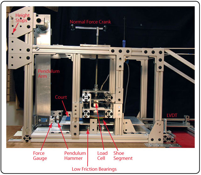
Figure 2 — Experimental Apparatus: Setup for measuring translational and rotational traction.
A 4.25-inch forefoot portion of a tennis shoe (Figure 3) is attached to a stationary mount (Asics Gel Resolution 6, size 9 U.S., right foot). This length approximates the location of the metarsal-phalangeal joint where the foot and shoe naturally flex during forefoot impact and push-off.
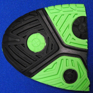
Figure 3 — A sample shoe test section.
The mounting structure can be raised and lowered to exert vertical forces from 0 to over 2200 N (500 lb) as measured by a load cell situated between the shoe mount and the force crank-down apparatus. A Decoturf (California Sports Surfaces) court surface was applied to a plexiglass backing and this is securely mounted on a 3/8-inch thick aluminum plate. This court surface ensemble is free to move linearly in one direction, gliding on a bed of low friction ball bearings with 360° freedom of motion (necessary for the rotational experiments). The shoe is oriented parallel to the direction of intended motion and lowered onto the court at a designated normal force. The aluminum plate containing the court surface is impacted by a weighted pendulum head with an effective mass of 3.1 kg. The impact energy can be altered by dropping the pendulum from any of six predetermined drop heights. The respective impact energies from lowest to highest were measured to be 2.3, 3.0, 4.1, 5.8, 9.5, and 16.0 J. The resulting impact force between the pendulum head and the court plate is measured by a force gauge located between the pendulum head and arm. A damping polymer is attached to the pendulum's impact face to limit high frequency vibration during impact with the aluminium court-holding plate (no signal filtering was performed). The linear distance travelled by the court under the shoe is measured by a linear variable differential transducer (LVDT) attached to the court. Figure 4 shows a schematic of this arrangement.
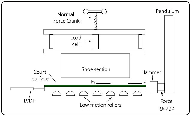
Figure 4 — Simplified view of the translational traction setup.
The setup for the rotational traction tests is exactly the same with two changes (Figure 5). First, the court section is smaller, rounded and has a hole drilled into it, which fits over a steel rod, around which the court will rotate. This axis of rotation is located directly under the forefoot section of the shoe and does not touch the shoe. The second difference is that the pendulum arm is moved to the side to impact the court eccentrically to the axis, causing rotation of the court under the shoe. The court has a pivoting impact appendage that the pendulum strikes. As the court rotates the appendage pivots to stay oriented flat against the pendulum hammer, keeping the force balanced on the force gauge. The court rotates clockwise to the right-foot shoe, equivalent to a medial, inward turn of the foot.
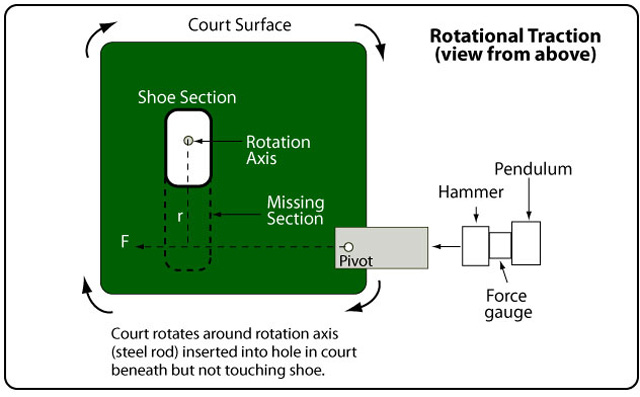
Figure 5 — Schematic of the rotational traction setup. It is exactly the same as the translational setup with three changes: (1) the court rotates around a steel rod axis under the forefoot section of the shoe, (2) the pendulum impacts the court off to the side at a distance equal to that between the axis of rotation and the middle of the heel of the shoe.
All traction testing devices must push the two surfaces together and make one surface move relative to the other. Either of the two surfaces can be made to move — the shoe and support structure can move relative to a stationary court fixture, or the court surface can move relative to the stationary shoe mount. Various methods have be used to implement both the vertical and horizontal forces.
Vertical force: To apply the vertical normal force some researchers have used weights [8-10, 23, 24] and others pneumatic rams or robotic motors [25, 16]. The essential task for applying normal loads is to test at several loads and to test at loads that are representative of loads exerted by players [26].
Horizontal force: To create relative movement of the surfaces a force is applied to one of the surfaces. That force might be implemented by hanging weights over a pully as Leonardo da Vinci did, or by using motors [8, 23, 24], pendulums horizontally striking one of the surfaces [9, 15], pneumatic actuators [21] or manual or vehicle-driven dragging [10]. There are two typical models of generating horizontal forces — (1) velocity or displacement controlled, as is common in most linear actuators, with the resulting force simply being the amount necessary to initiate the prescribed velocity or displacement between the surfaces; (2) force or impulse controlled, which is more realistic because it is a time-varying force that initiates the interaction and the relative court-shoe movement, should it occur. Another advantage of the latter method is that it can measure the initial resistance to movement and changes in shoe stiffness whereas velocity controlled tests only capture the peak traction values [27].
The testing for this current experiment fulfills the requirements for traction testing. The tests are performed at several tennis appropriate vertical and horizontal loads, and the horizontal loads can be classified as energy/force/impulse controlled actuations. The main limitation is that the horizontal force durations are much shorter than for actual foot contacts. The time to peak braking force in a running forehand is about 0.035 seconds [7] and the peak forces in the current tests were between 2-4 ms, or 10-20 times faster.
3. RESULTS AND DISCUSSION
(A) Translational Traction Results
Shear deformation and stiffness. The shoe (outsole and midsole forefoot section) and the court are pressed together by the applied normal force. Friction holds the two surfaces together, resisting relative motion. When the pendulum strikes the end of the court, it exerts a force that tries to move the court horizontally. This force increases up to some maximum. Traction resists and increases to match this applied force. As long as the traction force can increase to match the applied force, the shoe and court surface will remain stuck together and no sliding will occur. However, the shoe is softer than the court and will undergo shear deformation in the direction parallel to the applied force. The top side of the shoe is attached to the test rig and does not move, but the rest of the shoe deforms in the direction of motion. If the peak available traction force is not exceeded, the shoe and court will remain stuck together. If the peak available traction force is exceeded, bonds between the sole and the court will be broken and the court will slide. In either case, when the pendulum loses contact, the shear deformation will elastically recover and slide the court backward an equal amount (Figure 6).
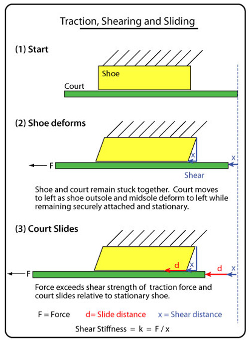
Figure 6 — The shoe will experience shear deformation in the direction of motion. The amount of shear will depend on the shear stiffness of the shoe outsole and midsole materials and may be as much as 2-5 mm. True sliding will be the distance recorded by the LVDT minus the shear distance.
Figure 7 shows two typical graphs of interaction between the two surfaces during the application of a dynamic tangential shear force. The LVDT records the court motion and the result is the sum of the shear deformation movement and the relative surface movement. The LVDT also records the elastic recovery of the deformation as the court moves backwards with the return to position of the shoe material after the force has terminated. This allows us to approximate how much of the total court movement was due to shoe deformation and how much to relative motion of the surfaces. The deformation will not be fully recovered, but it will be close. Two examples are shown in Figure 4 — in the first, traction holds and there is deformation (2.0 mm) but no sliding, and in the second there is deformation (1.7 mm) and sliding (4.1 mm). Recovered deformation is virtually 100% of the motion in the first example, whereas it is only a portion of the second example where sliding also occurs. Knowing the shear amount allows a calculation of the shear stiffness of shoe (Equation 4):
(4) k = Fave/ x
where k is the shear stiffness, Fave is the average applied force up to peak force (simply Fp / 2), and x is the shear deformation. (The effect of shear stiffness on traction will be discussed in the results section.)
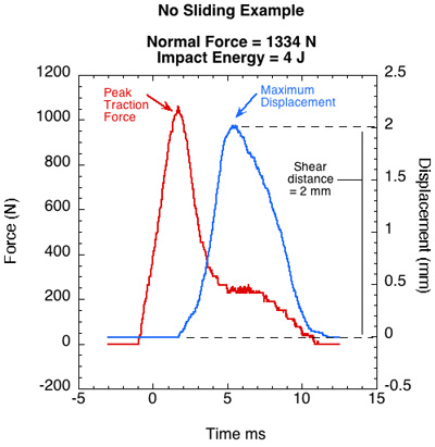
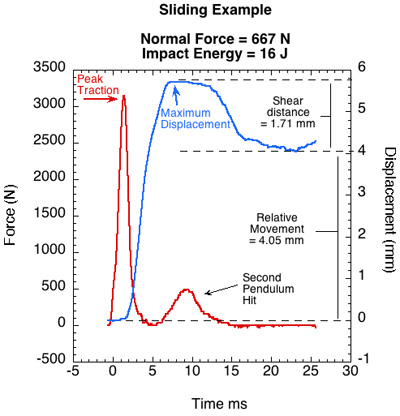
Figure 7— Graphic technique of determining the amount of shoe shear deformation (apparent movement between surfaces) compared to actual relative movement (sliding) between the surfaces.
The two surfaces begin sliding relative to each other at peak horizontal force and continue until the horizontal force is no longer large enough to overcome the dynamic friction between the sliding surfaces. (There is local micro-sliding prior to the peak force, with so-called rupture waves emanating from these slides and accumulating into gross sliding at the peak horizontal force, but that is beyond the scope of this study). The displacement curve will usually lag the force curve a bit because of the time-dependent shear deformation of the viscoelastic shoe section.
Normal force, peak traction force, and coefficient of traction. We are interested in how peak traction force and COT change as normal force and shear force change. As seen in Figure 8, for any given applied horizontal energy, peak traction force increases as normal force increases. And for any given normal force, traction increases with the magnitude of the applied energy.
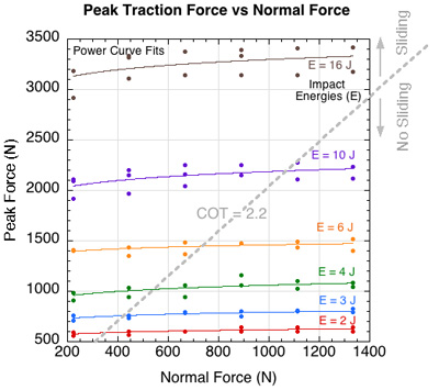
Figure 8 — For a given normal force, peak traction will increase with applied shear energy. For a given applied shear energy, traction will increase slightly with normal force. Above the dotted diagonal line (COT ≈ 2.2), sliding began subsequent to attainment of peak force, whereas there was no sliding subsequent to peak attainment below the line.
Traction increases both with increases in the normal force and the applied horizontal force. In the first case, the peak traction force increases more slowly than the normal force. That being the case, the denominator increases faster than the numerator in Equation 1, so COT decreases with increases in normal load. That result is demonstrated in Figure 9.
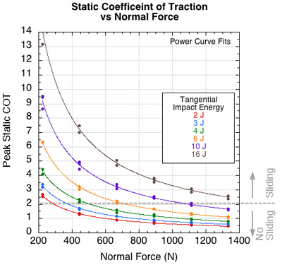
Figure 9 — For a given normal force, static COT increases with shear energy. For a given shear energy, static COT decreases with normal force. Above the dotted diagonal line (COT ≈ 2.2), sliding began subsequent to attainment of peak force and COT, whereas there was no sliding subsequent to peak attainment below the line.
This is consistent with previous investigations [22, 25, 28], though their results were for dynamic COT, not static COT. The COT curves all become asymptotic as the normal force increases. That reflects that fact that increase in real contact area between the surfaces begins to approach its maximum and the friction force increases very little with added normal force.
Loading rate and coefficient of traction. In Figure 3, the peak friction force increases very little as the normal force increases, but for any given normal force, peak friction force increases a great deal as the initiation energy increases. Increases in energy result in increased impact and friction reaction forces. Higher impact forces typically have shorter durations. The static COT depends heavily on the loading conditions of the event [29, 30]. One of these conditions is the shear force loading rate:
(5) dF/dt = Load Rate = Fp / tp
where Fp is the peak traction force and tp is the time from impact to peak force. For a given normal force, peak static COT depends on load rate (Figure 10).
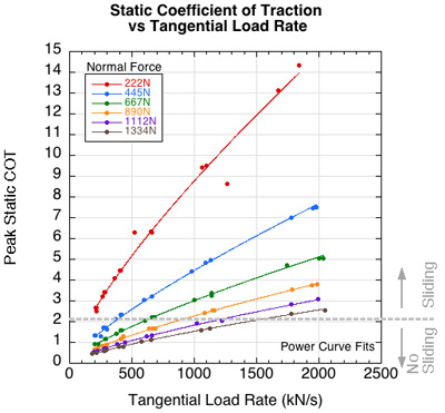
Figure 10 — For a given normal force, static COT increases with load rate, and for a given load rate, static COT decreases with an increase in normal force. Above the dotted diagonal line (COT ≈ 2.2), sliding began subsequent to attainment of peak force and COT, whereas there was no sliding subsequent to peak attainment below the line.
Sliding and coefficient of traction. Tennis players want enough friction to stop forward momentum and then push off and propel themselves to another location without slipping. Sometimes, instead, the player wishes to slide during the stopping phase. This is for two reasons: first because it is easier on the joints [28] and second because it allows for quicker repositioning [31]. Intentional sliding was once reserved for clay courts, but the technique (and the specially designed shoes) has recently been utilized on hard courts. Whatever the player's intent, he/she wants to know the likelihood that they will slip when they don't want to and will be able to slide when they want to. We want to know where on the available (static) COT curve sliding actually occurs. Figure 11 shows the distance that the court moved when hit by the impact pendulum.
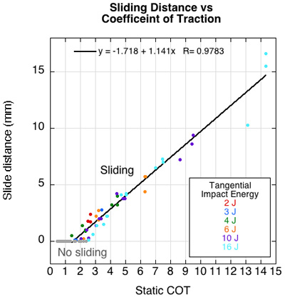
Figure 11 — Up to COT ≈ 2.0-2.5, there is no relative motion between the two sufaces. At COT >≈ 2 the shear elastic strength is exceeded and the surfaces begin to slide relative to each other.
This shoe exhibited maximum traction as long as the available COT was below 2.0-2.5. Above that the shoe would slide. In other words, the horizontal shear force had to exceed twice the normal force for the shoe to slip. That ratio may be quite typical of most tennis shoes, but it is far above the recommendations of many researchers.
The OSHA guideline for a safe work surface is > 0.5. The required static COT for normal to fast paced walking around obstacles has been shown to be between 0.38-0.54 [32, 33]. Other researchers have shown the correlation of lower extremity joint loading and traction [16, 28]. A maximum of COT = 0.8 has been recommended for athletic footwear by some [20, 34] and others have proposed lower between 0.5 and 0.7 [35]. It has also been shown that COT above 0.8 does not provide any marginal performance benefit [2]. It has been suggested that adding some slip to footwear could help prevent inury [21, 28].
Figure 12 shows how the peak force is reduced as shear deformation and sliding is increased. For a given horizontal energy the peak force goes down as sliding is increased, and sliding is increased by decreasing normal force. The way to alter the vertical and horizontal forces is to alter the angle of attack of the plant leg. But the way to increase sliding across all combinations of vertical and horizontal forces is to alter the traction mechanism between the shoe and surface. This is accomplished by shoe and court design.
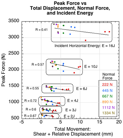
Figure 12 — Peak force varies with loading rate, normal force, and displacement distance.
Shoe Shear Stiffness. There was little correlation between COT and shear stiffness for impact energies of 2 and 3 J, but there was correlation for applied energies between 4-16 J. Figure 13 shows the latter. However, for the same applied energies between 4 and 16 J, shear stiffness was weakly and negatively correlated to normal force and positively correlated to applied energy (Figure 10b and 10c). Clarke et al. [21] found shear stiffness was positively correlated to normal force though also weakly. Given these weak and sometimes contrary causative relations of shear stiffness, along with the limited sample sizes for each parameter, the moderate correlation between COT and shear stiffness is inconclusive.
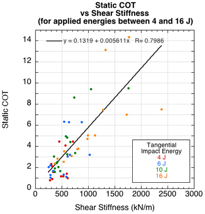
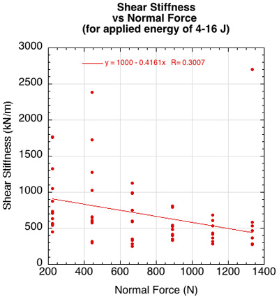
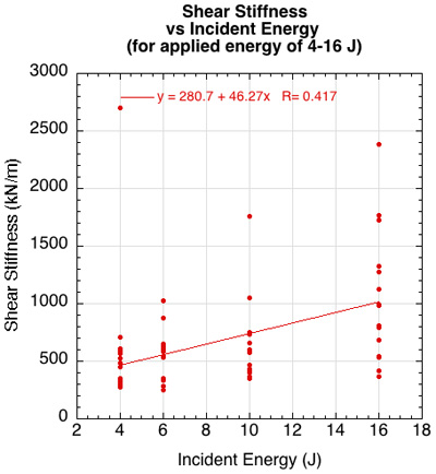
Figure 13 — (a) COT was correlated to shear stiffness for tangential force levels between 4J to 16J, while force levels below 4 J were not. (b) Shear force was weakly correlated to both normal force and (c) applied energy for applied energies between 4-16 J. Shear stiffness was negatively correlated to normal foce and positively to applied energy.
(B) Rotational Traction Results
The rotational traction tests were done at the same normal forces and applied horizontal energies, except that pendulum impacts at 2 and 3 J were eliminated. Figure 14 shows the peak torque attained at each normal force and for all applied energies. The torques for 4, 6, and 10 J of applied energy all mirror the results recorded in the field [15] for a running forehand.
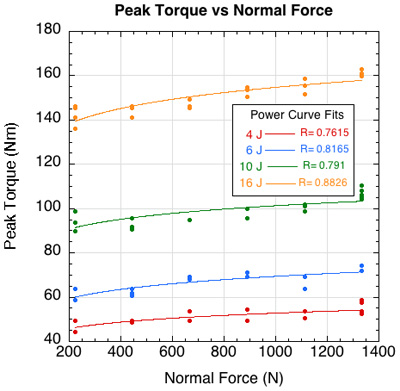
Figure 14 — Peak torque vs normal force.
Rotating a shoe is easier than sliding a shoe because the force is applied eccentrically and is facilitated by a lever (the moment arm of 120 mm). Just as with sliding, when the turning force is applied, the shoe begins to deform, this time across its width as opposed to its length in sliding. A some peak torque, the shoe and surface begin rotation relative to each other. The force with which this torque is achieved is much less than that which causes relative translational motion at the shoe-surface interface. As demonstrated in Figure 15 (as compared to Figure 8), this force is about 2.5 times less for rotational vs translational motion, for any given normal force and applied energy.
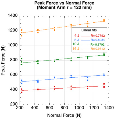
Figure 15 — Peak force vs normal force with moment arm equal to 120 mm.
Torque induced rotation angle was inversely related to normal force and positively related to applied horizontal energy (Figure 16)
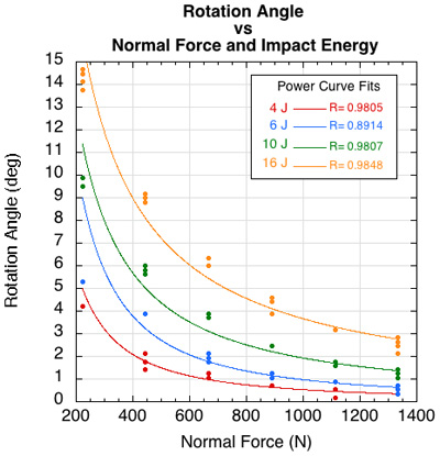
Figure 16 — Rotation angle vs normal force.
4. CONCLUSION
This study focused on the peak traction force developed between shoe and an acrylic hard court (US Open surface) and the various mechanisms that influence that force. This peak traction, as well as its traction coefficient (COT), are referred to as available traction and COT. These values were compared to the required or utilized traction necessary for a player to perform typical tennis maneuvers, as reported by several researchers. This comparison indicated that perhaps there is far more traction available than is necessary.
Traction is specific to the particular shoe-surface interface. Different surfaces will create different forces with the same shoe, and different shoes will create different forces with the same surface. These resultant traction forces are required for performance, but the open question is how much traction is required for tennis movements on a particular shoe-surface interface, how much is available, and how much is too much, contributing to many lower extremity injuries? It has been shown that players who play primarily on courts that allow sliding, like clay, also exhibit fewer injuries. But most players usually only have every day access to one type of court surface. Those players will want to play with the shoe that provides the most performance and least injury for that surface. At present, there is not enough research and data available to scientifically make those choices. The aim of this pilot study has been to identify and test parameters that will help us to make those choices.
The results indicate that peak traction force increases with normal force. The peak coefficient of traction (COT) decreases with normal force and increases with load rate. Sliding for this shoe occurs once COT is greater than about 2.0. Peak force lessened with more shear and sliding displacement and with lower normal force and load rate.
In retrospect, in this study, some of the tested normal forces were too low and horizontal forces too high as compared with values researchers have found existing in tennis movements. However, these latter studies are few and the forces occurring during sliding forehands on hard courts, for example, have not been adequately quantified. As such, the best range of test forces is still to be determined.
References
1. B. Barry and P. Milburn, “Tribology, friction and traction: understanding shoe-surface interaction,” Footwear Science 5(3), 137-145 (2013).
2. G. Luo and D. Stefanyshyn, “Identification of critical traction values for maximum athletic performance,” Footwear Science 3(3), 127-138 (2011).
3. B.N.J. Persson, “On the theory of rubber friction,” Surface Science 401, 445-454 (1998).
4. B.N.J. Persson, “Theory of rubber friction and contact mechanics,” Journal of Chemical Physics 115(8), 3840-3861 (2001).
5. L. Damm, D. Low, A. Richardson, J. Clarke, M. Carrre, and S. Dixon, “The effects of surface traction characteristics on frictional demand and kinematics in tennis,” Sports Biomechanics, 12-4, 389-402 (2013).
6. L. Damm, D. Low, A. Richardson, J. Clarke, M. Carre, and S. Dixon, “Modulation of tennis players’ frictional demand according to surface traction characteristics,” International Society of Biomechanics Congress XXIII, Brussels (2011).
7. V.H. Stiles and S.J. Dixon, “The influence of different playing surfaces on the biomechanics of a tennis running forehand foot plant,” Journal of Applied Biomechanics 22, 14-24 (2006).
8. G. Andreasson, U. Lindenberger, P.Renstrom, and L. Peterson, “Torque developed at simulated sliding between sport shoes and an artificial turf,” The American Journal of Sports Medicine 14(3), 225-230 (1986).
9. R.W. Bonstingl, C. A. Morehouse, and B.W. Niebel, “Torques developed by different types of shoes on various playing surfaces,” Medicine and Science in Sports 7(2), 127-131 (1975).
10. T.J. Serensits and A.S. McNitt, “Comparison of rotational traction of athletic footwear on varying playing surfaces using different normal loads,” Applied Turfgrass Science (2014).
11.R.S. Heidt, Jr., S.G. Dormer, P.W. Cawley, P.E. Scranton, Jr., G. Losse, and M. Howard, “Differences in friction and torsional resistance in athletic shoe-turf surface interfaces,” The American Journal of Sports Medicine, 834-842 (1996).
12. M. Shorten, B. Hudson, and J. Himmelsbach, “Shoe-surface traction of conventional and in-filled synthetic turf football surfaces,” In XIX International Congress of Biomechanics, New Zealand (2003).
13. M.R. Villwock, E.G. Meyer, J.W. Powell, A.J. Fouty, and R.C. Haut, “Football playing surface and shoe design affect rotational traction,” American Journal of Sports Medicine, 37(3), 518-525 (2009).
14. J.V. Dura, J.V. Hoyos, A. Martinez, and L. Lozano, “The influence of friction on sports surfaces in turning movements,” Sports Engineering, 2, 97-102 (1999).
15. B. Van Gheluwe and E. Deporte, “Friction measurement in tennis on the field and in the laboratory,” International Journal of Sport Biomechanics, 9, 48-61 (1992).
16. J.W. Wannop, J.T. Worobets, and D.J. Stefanyshyn, “Footwear traction and lower extremity loading,” The American Journal of Sports Medicine, Vol. XX, No. X.
17. D.J. Stefanyshyn and J.W. Wannop, “Biomechanics research and sport equipment development,” Sports Engineering 18, 191-202 (2015).
18. I.C. Wright, R.R. Neptune, A.J. van ben Bogert, and B.M. Nigg, “Passive regulation of impact forces in heel-toe running,” Clinical Biomechanics 13, 521-531 (1998).
19. E.M. Hennig, G.A. Valiant, and Q. Liu, “Biomechanical variables and the perception of cushioning for running in various types of footwear,” Journal of Applied Biomechanics 12, 143-150 (1996).
20. E.C. Frederick, “Optimal frictional properties for sport shoes and sport surfaces,” In 11 International Symposium on Biomechanics in Sports, (1993).
21. J. Clarke, M. Carre, L. Damm, and S. Dixon, “The development of an apparatus to understand the traction developed at the shoe-surface interface in tennis,” Proceedings of the Institution of Mechanical Engineers, Part P: Journal of Sports Engineering and Technology 227 (3), 149-160 (2013).
22. J. Clarke, M. Carre, L. Damm, and S. Dixon, “Understanding the influence of surface roughness on the tribological interactions at the shoe-surface interface in tennis,” J. Engineering Tribology 226(7), 636-647 (2012).
23. M.A. Chowduhury, M.K. Khalil, D.M. Nuruzzaman, and M.L. Rahaman, “The effect of sliding speed and normal load on friction and wear property of aluminum,” International Journal of Mechanical and Mechatronics Engineering 11(01), 45-49 (2011).
24. M.S. Redfern, A. Marcotte, and D.B. Chaffin, “A dynamic coefficient of friction measurement device for shoe/floor interface testing,” Journal of Safety Research 21, 61-65, (1990).
25. J. Clarke, M. Carre, A. Richardson, Z. Yang, L. Damm, and S. Dixon, “Understanding the traction of tennis surfaces,” Procedia Engineering 13, 402-408 (2011).
26. B.M. Nigg, “The validity and relevance of tests used for the assessment of sports surfaces,” Medicine & Science in Sports & Exercise, (1990).
27. M. Carre, B. Kirk, and S. Haake, “Developing relevant tests for traction of studded footwear on surfaces,” http://sportsurf.lboro.ac.uk/workshops/STARSS/S1/MC.pdf [cited 6/13/16].
28. B.M. Nigg, “Injury and performance on tennis surfaces: the effect of tennis surfaces on the game of tennis,” http://hartru.com/uploads/downloads/Doc_7.pdf (2003) [cited 7/19/16].
29. O. Ben-David and J. Fineberg, “The dynamics of the onset of frictional slip,” Science (October 2010).
30. O. Ben-David and J. Fineberg, “Static friction coefficient is not a material constant,” Physical Review Letters 106.254301 (June, 2011).
31. S. Pavailler and N. Horvais, “Sliding allows faster repositioning during tennis specific movements on hard court,” Procedia Engineering 72(2014), 859-864 (2014).
32. P. Fino and T. Lockhart, “Required coefficient of friction during turning as self-selected slow, normal, and fast walking speeds,” J Biomech 47(6), 1395-1400 (2014).
33. J.M. Burnfield, C.D. Few, J. Tsai, and C.M. Powers, “Prediction of peak utilized coefficient of friction requirements during walking based on center of mass kinematics,” Proceedings International Society of Biomechanics XIXth Congress (2003).
34. G.A. Valiant, “The relationship between normal pressure and the friction developed by shoe outsole material on a court surface,” Journal of Biomechanics 20(9), 892 (1987).
35. B.M. Nigg and B. Segesser, “The influence of playing surfaces on the load on the locomotor system and on football and tennis injuries,” Sports Med. 5(6), 375-85 (1988).